Question

Problem #4. The convective heat transfer problem of cold oil flowing over a hot surface can be described by the following second-order ordinary differential equations. der 0 dx T(0)=0 (1) T(5)=1 where T is the dimensionless temperature and x is the dimensionless similarity variable. dr? +0.83, dT This is a boundary-value problem with the two conditions given on the wall (x=0, T(O) = 0) and in the fluid far away from the wall (x = 5,7/5) = 1). You are asked to use the shooting method to solve this problem by employing the MATLAB functions such as ode45 and fzero: 4.1 First, convert this second-order ordinary differential equation into two first-order ordinary differential equations for function yr and yz, y = 7 4.2 dT Y2= dx On a white paper, write down the two first-order ordinary differential equations with the corresponding conditions. Set up the function file, [dy] = dTdx (x,y), so that the two first-order ordinary differential equations can be solved by using the MATLAB ODE solver, "ode 45" of initial value ODES. Construct the residual function file, [r] = residual (2a), so that MATLAB "zero" of root-finding can be used to find the required y(O) for the present boundary-value problem. Make a plot the solution of T vs x. 4.3 4.4

Answer 1

-0.83 x² % 4.1 T" +0.838²7"=0 g) T" = -0.83%? T' T(0)=0, T(s) = 1 Assume, YT Y2 = T' y = T'=% yo -- [] > 0.83x2y2 D' Y, (o)= 0, y, 1) = 1

%% 4.2
function dy = dTdx( x, y )

dy = [y(2); -0.83*x^2*y(2) ];

end

%% 4.3
function r = residual( za )
global L y1_5 y1_0
[~,y] = ode45(@dTdx,[0,L],[y1_0,za]);
r = y(end,1)-y1_5;
end

%% 4.3
clc
clear all

global L y1_5 y1_0
L = 5; % dimensionless variable
y1_5 = 1;
y1_0 = 0;

y2_0 = fzero(@residual,[0,10]);

%% 4.4
[x,y]=ode45(@dTdx,[0 L],[y1_0, y2_0]);

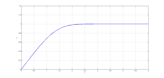
plot(x,y(:,1),'LineWidth',2);
xlabel('x');
ylabel('T');
grid on

1.4 1.24 0.8 0.6 0.41 0.21 0.5 1.5 12 3.5 4.5 5 2.5 x