


Homework Answers
ANSWER:
a)
For the given data
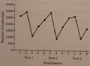
The time series plot is
By using excel

| SUMMARY OUTPUT | |||||||
| Regression Statistics | |||||||
| Multiple R | 0.989744 | ||||||
| R Square | 0.979592 | ||||||
| Adjusted R Square | 0.971939 | ||||||
| Standard Error | 124.9667 | ||||||
| Observations | 12 | ||||||
| ANOVA | |||||||
| df | SS | MS | F | Significance F | |||
| Regression | 3 | 5996942 | 1998981 | 128.003 | 4.23E-07 | ||
| Residual | 8 | 124933.3 | 15616.67 | ||||
| Total | 11 | 6121875 | |||||
| Coefficients | Standard Error | t Stat | P-value | Lower 95% | Upper 95% | Lower 95.0% | |
| Intercept | 2492 | 72.14954 | 34.53476 | 5.4E-10 | 2325.29 | 2658.044 | 2325.29 |
| x1 | -712 | 102.0349 | -6.97474 | 0.000116 | -946.959 | -476.374 | -946.959 |
| x2 | -1512 | 102.0349 | -14.8152 | 4.24E-07 | -1746.96 | -1276.37 | -1746.96 |
| x3 | 327 | 102.0349 | 3.20152 | 0.012584 | 91.37388 | 561.9595 | 91.37388 |
From the above
| Coefficients | |
| Intercept | 2492 |
| x1 | -712 |
| x2 | -1512 |
| x3 | 327 |
b)
y = 2492 -712 x1 - 1512 x2 + 327 x3
c)
| Quarter 1 forecast | y =2492 -712 (1) - 1512 (0)+ 327 (0) | 1780 |
| Quarter 2 forecast | y =2492 -712 (0) - 1512 (1)+ 327 (0) | 980 |
| Quarter 3 forecast | y =2492 -712 (0) - 1512 (0)+ 327 (1) | 2818 |
| Quarter 4 forecast | y =2492 -712 (0) - 1512 (0)+ 327 (0) | 2492 |
d)
| y | t | SUMMARY OUTPUT | ||||||||
| 1690 | 1 | |||||||||
| 940 | 2 | Regression Statistics | ||||||||
| 2625 | 3 | Multiple R | 0.301477 | |||||||
| 2500 | 4 | R Square | 0.090889 | |||||||
| 1800 | 5 | Adjusted R Square | -2.3E-05 | |||||||
| 900 | 6 | Standard Error | 746.0205 | |||||||
| 2900 | 7 | Observations | 12 | |||||||
| 2360 | 8 | |||||||||
| 1850 | 9 | ANOVA | ||||||||
| 1100 | 10 | df | SS | MS | F | Significance F | ||||
| 2930 | 11 | Regression | 1 | 556408.4 | 556408.4 | 0.999752 | 0.34095 | |||
| 2615 | 12 | Residual | 10 | 5565467 | 556546.7 | |||||
| Total | 11 | 6121875 | ||||||||
| Coefficients | Standard Error | t Stat | P-value | Lower 95% | Upper 95% | Lower 95.0% | ||||
| Intercept | 1612 | 459.1439 | 3.510981 | 0.005622 | 589.0091 | 2635.082 | 589.0091 | |||
| t | 62 | 62.38537 | 0.999876 | 0.34095 | -76.6256 | 201.3809 | -76.6256 |
y = 1612 + 62 t
Forecast
year 4
| Quarter 1 | y = 1612 + 62 (13) | 2418 |
| Quarter 2 | y = 1612 + 62 (14) | 2480 |
| Quarter 3 | y = 1612 + 62 (15) | 2542 |
| Quarter 4 | y = 1612 + 62 (16) | 2604 |
If you have any doubts please comment and please don't dislike.
PLEASE GIVE ME A LIKE. ITS VERY IMPORTANT FOR ME.
Add Answer to:
Please help. I'm stuck.
The quarterly sales data (number of copies sold) for a college textbook...
6. eBook The quarterly sales data (number of copies sold) for a college textbook over the past th...
 6. eBook The quarterly sales data (number of copies sold) for a college textbook over the past three years follow Quarter Year 1 Year 2 Year 3 1,765 1,063 2,974 2,554 1,591 1,827 935 2,646 2,423 980 2,812 2,358 4 There appears to be a seasonal pattern in the data and perhaps amoderate upward linear trend b. Use the following dummy variables to develop an estimated regression equation to account for any seasonal effects in the data: Qtrl 1 if...
The quarterly sales data (number of book sold) for Christian book over the past three years...
The quarterly sales data (number of book sold) for Christian book over the past three years in California follow: (You can use Excel to compute the equation) Quarter Year 1 Year 2 Year 3 1 2 3 4 1230 1020 2534 2600 1470 990 2800 2590 1520 1020 2850 2700 1. Use the following dummy variables to develop an estimated regression equation to account for any seasonal effects in the data: Quarter1=1 if the sales data point is in Quarter...
Please help I am very confused on how to solve this South Shore Construction builds permanent...
 Please help I am very confused on how to
solve this
South Shore Construction builds permanent docks and seawalls along the southern shore of Long Island, New York. Although the firm has been in business only five years, revenue has increased from $315,000 in the first year of operation to $1,075,000 in the most recent year. The following data show the quarterly sales revenue in thousands of dollars. Quarter Year 1 TE Year 2 Year 3 Year 4 Year 5...
Please help I am very confused on how to
solve this
South Shore Construction builds permanent docks and seawalls along the southern shore of Long Island, New York. Although the firm has been in business only five years, revenue has increased from $315,000 in the first year of operation to $1,075,000 in the most recent year. The following data show the quarterly sales revenue in thousands of dollars. Quarter Year 1 TE Year 2 Year 3 Year 4 Year 5...
Quarter Year 1 Year 2 Year 3 Year 4 Year 5 1 20 42 69 98...
 Quarter
Year 1
Year 2
Year 3
Year 4
Year 5
1
20
42
69
98
175
2
101
141
149
211
288
3
168
250
333
388
436
4
6
20
47
91
181
South Shore Construction builds permanent docks and seawalls along the southern shore of Long Island, New York. Although the firm has been in business only five years, revenue has increased from $295,000 in the first year of operation to $1,080,000 in the most recent year....
Quarter
Year 1
Year 2
Year 3
Year 4
Year 5
1
20
42
69
98
175
2
101
141
149
211
288
3
168
250
333
388
436
4
6
20
47
91
181
South Shore Construction builds permanent docks and seawalls along the southern shore of Long Island, New York. Although the firm has been in business only five years, revenue has increased from $295,000 in the first year of operation to $1,080,000 in the most recent year....
Six years of quarterly data of a seasonally adjusted series are used to estimate a linear...
 Six years of quarterly data of a seasonally adjusted series are used to estimate a linear trend model as T = 164.90 +1.09. In addition, quarterly seasonal indices are calculated as $ 1-0.88, Ŝ 2=0.94, § 3 = 116, and § 4 = 1.12. b. Make a forecast for all four quarters of next year. (Do not round intermediate calculations. Round your answers to 2 decimal places.) 169.09 Quarter 1 Quarter 2 Quarter 3 Quarter 4
Problem 15-28 (Algorithmic) South Shore Construction builds permanent docks and seawalls along the southern shore of...
Problem 15-28 (Algorithmic) South Shore Construction builds permanent docks and seawalls along the southern shore of long island, new york. Although the firm has been in business for only five years, revenue has increased from $400,000 in the first year of operation to $1,092,000 in the most recent year. The following data show the quarterly sales revenue in thousands of dollars: Quarter Year 1 Year 2 Year 3 Year 4 Year 5 1 43 46 75 99 178 2 123...
Q6 3 4 91 Q6. The following data show the quarterly sales of Amazing Graphics, Inc....
 Q6
3 4 91 Q6. The following data show the quarterly sales of Amazing Graphics, Inc. for the years 1 through 3. Year Quarter Time Period (t) Sales (1000s) 1 2 4.1 6.0 6.5 5.8 5.2 6.8 7.4 3 6.0 510 5.6 13 3 117.5 13 128.8 From the above data, it could be concluded that both quarterly seasonal effects and linear trend in the sales pattern are present. A time series model was considered for this question and the...
Q6
3 4 91 Q6. The following data show the quarterly sales of Amazing Graphics, Inc. for the years 1 through 3. Year Quarter Time Period (t) Sales (1000s) 1 2 4.1 6.0 6.5 5.8 5.2 6.8 7.4 3 6.0 510 5.6 13 3 117.5 13 128.8 From the above data, it could be concluded that both quarterly seasonal effects and linear trend in the sales pattern are present. A time series model was considered for this question and the...
Six years of quarterly data of a seasonally adjusted series are used to estimate a linear...
 Six years of quarterly data of a seasonally adjusted series are used to estimate a linear trend model as T1 = 194.40 + 1.23t. In addition, quarterly seasonal indices are calculated as S, = 0.94, S2 = 0.88, S3 = 1.20, and S4 = 1.02. a-1. Interpret the first quarterly index. In other words, what is the value of the series in the first quarter as compared to the average? 94% below O 6% above 94% above 6% below a-2....
The quarterly sales in units for “Retailsale Sports” for the last two years are as follows:...
The quarterly sales in units for “Retailsale Sports” for the last two years are as follows: Quarter Year 1 Year 2 I 440 560 II 460 490 III 420 500 IV 390 400 Using linear regression, a straight line was fitted to the sales data. Assume that the equation of the fitted line is Y = 420 + 6 × t. The first quarter in the data is labeled t = 1. Calculate seasonal indexes for this product using the...
 6. eBook The quarterly sales data (number of copies sold) for a college textbook over the past three years follow Quarter Year 1 Year 2 Year 3 1,765 1,063 2,974 2,554 1,591 1,827 935 2,646 2,423 980 2,812 2,358 4 There appears to be a seasonal pattern in the data and perhaps amoderate upward linear trend b. Use the following dummy variables to develop an estimated regression equation to account for any seasonal effects in the data: Qtrl 1 if...
 Please help I am very confused on how to
solve this
South Shore Construction builds permanent docks and seawalls along the southern shore of Long Island, New York. Although the firm has been in business only five years, revenue has increased from $315,000 in the first year of operation to $1,075,000 in the most recent year. The following data show the quarterly sales revenue in thousands of dollars. Quarter Year 1 TE Year 2 Year 3 Year 4 Year 5...
Please help I am very confused on how to
solve this
South Shore Construction builds permanent docks and seawalls along the southern shore of Long Island, New York. Although the firm has been in business only five years, revenue has increased from $315,000 in the first year of operation to $1,075,000 in the most recent year. The following data show the quarterly sales revenue in thousands of dollars. Quarter Year 1 TE Year 2 Year 3 Year 4 Year 5...
 Quarter
Year 1
Year 2
Year 3
Year 4
Year 5
1
20
42
69
98
175
2
101
141
149
211
288
3
168
250
333
388
436
4
6
20
47
91
181
South Shore Construction builds permanent docks and seawalls along the southern shore of Long Island, New York. Although the firm has been in business only five years, revenue has increased from $295,000 in the first year of operation to $1,080,000 in the most recent year....
Quarter
Year 1
Year 2
Year 3
Year 4
Year 5
1
20
42
69
98
175
2
101
141
149
211
288
3
168
250
333
388
436
4
6
20
47
91
181
South Shore Construction builds permanent docks and seawalls along the southern shore of Long Island, New York. Although the firm has been in business only five years, revenue has increased from $295,000 in the first year of operation to $1,080,000 in the most recent year....
 Six years of quarterly data of a seasonally adjusted series are used to estimate a linear trend model as T = 164.90 +1.09. In addition, quarterly seasonal indices are calculated as $ 1-0.88, Ŝ 2=0.94, § 3 = 116, and § 4 = 1.12. b. Make a forecast for all four quarters of next year. (Do not round intermediate calculations. Round your answers to 2 decimal places.) 169.09 Quarter 1 Quarter 2 Quarter 3 Quarter 4
 Q6
3 4 91 Q6. The following data show the quarterly sales of Amazing Graphics, Inc. for the years 1 through 3. Year Quarter Time Period (t) Sales (1000s) 1 2 4.1 6.0 6.5 5.8 5.2 6.8 7.4 3 6.0 510 5.6 13 3 117.5 13 128.8 From the above data, it could be concluded that both quarterly seasonal effects and linear trend in the sales pattern are present. A time series model was considered for this question and the...
Q6
3 4 91 Q6. The following data show the quarterly sales of Amazing Graphics, Inc. for the years 1 through 3. Year Quarter Time Period (t) Sales (1000s) 1 2 4.1 6.0 6.5 5.8 5.2 6.8 7.4 3 6.0 510 5.6 13 3 117.5 13 128.8 From the above data, it could be concluded that both quarterly seasonal effects and linear trend in the sales pattern are present. A time series model was considered for this question and the...
 Six years of quarterly data of a seasonally adjusted series are used to estimate a linear trend model as T1 = 194.40 + 1.23t. In addition, quarterly seasonal indices are calculated as S, = 0.94, S2 = 0.88, S3 = 1.20, and S4 = 1.02. a-1. Interpret the first quarterly index. In other words, what is the value of the series in the first quarter as compared to the average? 94% below O 6% above 94% above 6% below a-2....
Most questions answered within 3 hours.
-
Write in C++
Name sort
Write a program that allows you to input up to 20...
asked 28 seconds ago -
An individual who has automobile insurance from a certain
company is randomly selected. Let Y be...
asked 17 minutes ago -
Initial mean=6600 and median = 1500, after 2 data sets removed,
new mean = 1850 and...
asked 19 minutes ago -
A 3330-kg spacecraft is in a circular orbit 2770 km above the
surface of Mars.
How...
asked 18 minutes ago -
The outcome X of an experiment has only two possible values, X=4
and X=5. Given that...
asked 19 minutes ago -
When UV light of wavelength 288 nm falls on a metal surface, the
maximum kinetic energy...
asked 29 minutes ago -
Your company has just brought in a new line of products... And
they are pieces of...
asked 33 minutes ago -
in three paragraphs or more discuss the role of the U.S.
Children’s Bureau in dealing with...
asked 32 minutes ago -
Place the following salts in order of increasing water
solubility:
i. Fe(OH)2 Ksp = 7.9 ×...
asked 35 minutes ago -
If inflation is increasing at 2.6 percent per year, and your
salary increases at the same...
asked 36 minutes ago -
An aspirin dose of 5.0mg per kg of body weight has been
prescribed to reduce the...
asked 42 minutes ago -
The AASB Conceptual Framework (2.12-2.19) refers to ‘faithful
representation’ as being necessary for financial information to...
asked 47 minutes ago