Question

6.40 Determine and plot, for the system of Figure P6.40, its response i(1) (a) when y(t) = 106(1), (b) when v(t) = 10u(t), and (c) when v(t) = 0.51. 0.2 H VO 2.60 0.1 uF FIG. P6.40

Answer 1

044 - 2.6 +0.145 0.145 6:40 Applying KVL; we get; V() = 0.2 g + 2.6i + xi(t) at - applying Laplace tram form; we get; + N(S) = 0.25 I(S) + 2.6 I(S) + I(S) = + 028) 375) 1+ 2.6*0.1X106S+0.2x 01x10-652 + V(S) = x I(S) 0.1810-6xg therefore, I (S) 0.1810 6xg 55. V(s) 0.280.181068² + 2.6X0.1X1065 +1 S²+ 135+ 5x107 The following matlas Code Can be wad & to get the response of (t); cohen () (+) - 0.51 a) V(t) = 10 () b) v(t) = 10 u(+) =

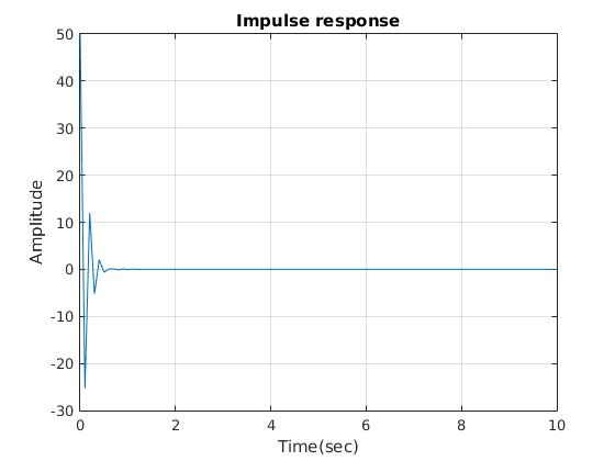
a) for v(t) = 10*delta(t); the matlab code and plot are shown below

clear all
clc
s = tf('s');
%% model the system
R = 2.6; % in ohm
L = 0.2; % in Henry
C = 0.1e-06; % in microFarad
% model the trnasfer function
G = (s/L)/(s^2 + (R/L)*s + (1/(L*C)));

%% compute response and plot
time = 0:0.1:10; % time of simulation
% a) v(t) = 10*delta(t)
[y_im,t_im] = impulse(G,time);
% plot the response
figure(1)
plot(t_im,10*y_im)
grid
xlabel('Time(sec)')
ylabel('Amplitude')
title('Impulse response')

Impulse response 50 40 30 20 Amplitude 10 O -10 -20 -30 0 4 8 10 IN 6 Time(sec)

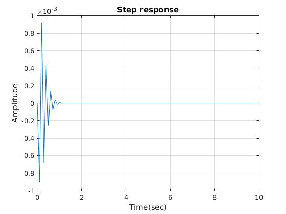
b) for v(t) = 10*u(t); the matlab code and plot are shown below

% b) v(t) = 10*u(t)
u = 10*ones(1,length(time));
[y_step,t_step] = lsim(G,u,time);
% plot the response
figure(2)
plot(t_step,y_step)
grid
xlabel('Time(sec)')
ylabel('Amplitude')
title('Step response')

The response is shown below

*103 Step response 1 0.8 0.6 0.4 0.2 Amplitude 0 -0.2 -0.4 -0.6 -0.8 -1 4 8 10 IN 6 Time(sec)

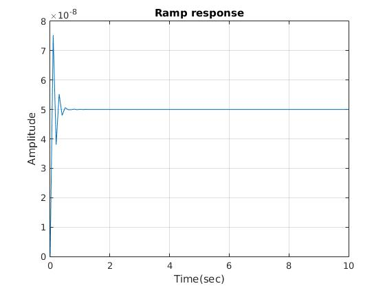
c) for v(t) = 0.5*t; the matlab code and plot are shown below

% c) v(t) = 0.5*t
u_ramp = 0.5*time.*ones(1,length(time));
[y_ramp,t_ramp] = lsim(G,u_ramp,time);
% plot the response
figure(3)
plot(t_ramp,y_ramp)
grid
xlabel('Time(sec)')
ylabel('Amplitude')
title('Ramp response')

The corresponding response is shown below

10-8 Ramp response 8 7 6 5 Amplitude 3 N 1 0 4 8 10 IN 6 Time(sec)