Question

solve it with matlab

25.24 Given the initial conditions, y(0) = 1 and y'(0) = 1 and y'(0) = 0, solve the following initial-value problem from t = 0 to 4: dy + 4y = 0 dt² Obtain your solutions with (a) Euler's method and (b) the fourth- order RK method. In both cases, use a step size of 0.125. Plot both solutions on the same graph along with the exact solution y = cos 2t.

Answer 1

`Hey,

Note: If you have any queries related to the answer please do comment. I would be very happy to resolve all your queries.

clc

clear all

close all

format long

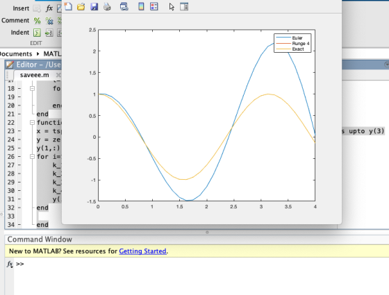
f=@(t,y) [y(2);-4*y(1)];

[T1,Y1]=eulerSystem(f,[0,4],[1,0],0.125);

f=@(t,y) [y(2),-4*y(1)];

[T2,Y2]=runge4(f,[0,4],[1,0],0.125);

plot(T1,Y1(1,:),T2,Y2(:,1),T1,cos(2*T1));

legend('Euler','Runge 4','Exact');

function [t,y]=eulerSystem(Func,Tspan,Y0,h)

t0=Tspan(1);

tf=Tspan(2);

N=(tf-t0)/h;

y=zeros(length(Y0),N+1);

y(:,1)=Y0;

t=t0:h:tf;

for i=1:N

y(:,i+1)=y(:,i)+h*Func(t(i),y(:,i));

end

end

function [x,y]=runge4(f,tspan,y0,h)

x = tspan(1):h:tspan(2); % Calculates upto y(3)

y = zeros(length(x),2);

y(1,:) = y0; % initial condition

for i=1:(length(x)-1) % calculation loop

k_1 = f(x(i),y(i,:));

k_2 = f(x(i)+0.5*h,y(i,:)+0.5*h*k_1);

k_3 = f((x(i)+0.5*h),(y(i,:)+0.5*h*k_2));

k_4 = f((x(i)+h),(y(i,:)+k_3*h));

y(i+1,:) = y(i,:) + (1/6)*(k_1+2*k_2+2*k_3+k_4)*h; % main equation

end

end

M Insert fx & Comment % 92% Indent 2.5 EDIT Euler Runge 4 Exact 2. Documents MATL Editor - /Use saveee.m 1.5 - fo 18 19 20 21 22 23 0.5 en end functi X = tsi y = ze y(1,:) for i=1 5 upto y(3) 24 - 0 25 - 26 27 -0.5 28 -1 29 30 31 32 - 33 34 - yo end -1.5 0 0.5 1 1.5 2 2.5 3 3.5 4 end Command Window New to MATLAB? See resources for Getting Started.

Kindly revert for any queries

Thanks.