Question

Use Matlab to plot two cycles of the following ) waveforms: a. yi(t) = sin(200m) volts b· pd) =-1.0+ cos(2000m) volts c. y)--1.0 to 3.0 volt square wave at 1,000 Hz Then use Matlab to compute the max, min, average, and rms values for each of the signals listed above.

Answer 1

clear
clc
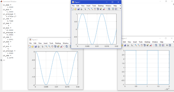
%y1
period=2/200;
t=linspace(0,2*period,1000);
y1=sin(200*pi*t);
figure
plot(t,y1)
grid on
y1_max=max(y1)
y1_min=min(y1)
y1_average=mean(y1)
y1_rms=rms(y1)
%y2
period=2/200;
t=linspace(0,2*period,1000);
y2=-1+cos(200*pi*t);
figure
plot(t,y2)
grid on
y2_max=max(y2)
y2_min=min(y2)
y2_average=mean(y2)
y2_rms=rms(y2)
%y3
f=1000;
period=1/1000;
t=linspace(0,2*period,1000);
y3=1+2*square(2*pi*f*t);
figure
plot(t,y3)
grid on
y3_max=max(y3)
y3_min=min(y3)
y3_average=mean(y3)
y3_rms=rms(y3)