Question

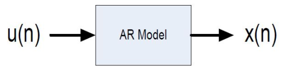
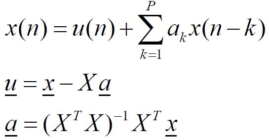
It is decided to use an AR model (a linear prediction model) of an observed signal x(n) in order to estimate the
signal’s power spectral density. The model linear prediction parameters will be determined using least squares
analysis, based on the equations:

u (n) AR Model x(n)

1. In a particular experiment we observe x(n) = 1.0, 1.1, 1.2, 1.3, 1.4, 1.5, 1.6, 1.7, 1.8, 1.9 for n = 0, 1, 2, 3, 4,
5, 6, 7, 8, 9 respectively. Fill in specific numeric values for the vector x and the matrix X in the above equations,
assuming that we want to use the available data (only the available data described) to compute the coefficients
a for a linear prediction model with P = 4.

2. Assume that after correctly performing the least squares solution above, you get the result:

                    a = [ 1.2 -0.4 0.6 -0.2]

Write out the explicit Z-domain transfer function HAR(z) for the above signal model, where X(z) = Har(z) U(z).
Be sure to include the specific numerical coefficients rather than generic symbolic coefficients.
                   Har(z) =

3. It is desired to use the MATLAB freqz() function to estimate the frequency response Har(w) of the filter in
the AR model, where w represents normalized frequency in radians. This MATLAB function has the general
form:
                    [Har, w] = freqz(B, A, N);

Where B is a vector representing the numerator of Har(z), A is a vector representing the denominator of Har(z),
and N is the number of points at which you want to evaluate Har(w) (evenly spaced between w = 0 and the
Nyquist frequency w=pi). In the MATLAB result, Har is the vector of computed frequency responses and w is
the corresponding vector of normalized frequencies. Fill in the actual vector numeric values for the MATLAB
variables B and A, assuming the specific AR model solution in part b above.

                    B =[                     ]      A=[          ]

4. It is desired to use the MATLAB filter() and var() functions to estimate the variance of the AR model’s
hypothetical input function u(n) assuming the specific AR model solution in part b above. These functions have
the general form:
                     u = filter(Bu, Au, x);
                     var_u = var(u);

Where Bu is a vector representing the numerator of Hu(z), and Au is a vector representing the denominator of
Hu(z), where U(z) = Hu(z) X(z). Fill in the actual vector numeric values for Bu and Au, assuming the AR model
solution in part b above.

                      Bu =[ ]             Au =[                       ]

5.    It is desired to use the MATLAB semilogy() function to display the estimate of the power spectral density of
the observed signal x, based on the AR model formulated above. This function has the general form:

                     semilogy(w, Pxx);

Where Pxx is a vector representing the power spectral density of x estimated at the normalized frequencies in
the vector w. Complete the MATLAB expression to compute Pxx based on Har and var_u as computed in parts
3. and 4. above.

                      Pxx =

Answer 1

D = fdesign.lowpass('Nb, Na, F3dB', 10,10,0.2): OPTS = design opts(D, 'butter') if(OPTS.Filter Structure = = 'df2s0s') f printf('The default filter structure is Direct-Form II\n'): f printf('with second-order sections.\n'): end OPTS = struct with fields: Filter Structure: 'df2sos' SOSScaleNorm: '' SOSScaleopts: [1 times 1 fdopts.sosscaling] System object: theta The default filter structure is Direct-Form II with second-order sections. N = 0: 159: x = cos(pi/8*n) + 0.25*sin(pi/4*n): y = filter(Hd, x): Plot the original and filtered signals in the frequency domain. freq = 0: (2*pi)/160: pi: xdft = fft(x): ydft = fft(y): plot(freq/pi, abs(xdft(1: length(x)/2 + l))) hold on plot (f req/pi, abs (ydft (1: length (y)/2 + l)),' r',' linewidth' ,2) hold off legend(' Original Signal',' Low pass Signal',' Location',' NorthEast') y label('Magnitude*) x label('Normalized Frequency (\times\pi rad/sample)')