Question

-Conduct a Linear regression

-Describe the results of the linear regression

Average US Gas Price 1991-2015 (in dollars per gallon) Year Average US Gas Price 2 Period Moving Average 3 Period Moving Average 1991 1992 1993 1994 1995 1996 1997 1998 1999 2000 2001 2002 2003 2004 2005 2006 2007 2008 2009 2010 2011 2012 2013 2014 2015 1.14 N/A 1.13 1.11 1.11 1.15 1.23 1.23 1.06 1.17 1.51 N/A 1.135 N/A 1.127 1.36 1.59 1.88 2.3 2.59 2.8 3.27 2.35 2.79 3.53 3.64 3.53 3.37 2.45 1.12 1.11 1.13 1.19 1.23 1.145 1.115 1.34 1.485 1.41 1.475 1.735 2.09 2.445 2.695 3.035 2.81 2.57 3.16 3.585 3.585 3.45 2.91 1.123 1.163 1.203 1.173 1.153 1.247 1.38 1.443 1.47 1.61 1.923 2.257 2.563 2.887 2.807 2.803 2.89 3.32 3.567 3.513

Answer 1

Answer

Data set for the regression analysis is given below

Year	Average US gas price
1991	1.14
1992	1.13
1993	1.11
1994	1.11
1995	1.15
1996	1.23
1997	1.23
1998	1.06
1999	1.17
2000	1.51
2001	1.46
2002	1.36
2003	1.59
2004	1.88
2005	2.3
2006	2.59
2007	2.8
2008	3.27
2009	2.35
2010	2.79
2011	3.53
2012	3.64
2013	3.53
2014	3.37
2015	2.45

Using Excel, go to Data analysis, then select Regression

select Average US gas price as input y range and year as input x range, then click OK

we will the get the following Regression output

SUMMARY OUTPUT Regression Statistics MultipleR R Square Adjusted R Square Standard Error Observations 0.8995 0.8090 0.8007 0.4131 25.0000 ANOVA MS Significance F Regression Residual Total 1.0000 23.0000 24.0000 16.6268 3.9244 20.5512 16.6268 97.4468 0.0000 0.1706 Coefficients Standard Error 22.9474 0.0115 P-value Lower 95% Upper 95% Lower 95.0% 236-271.9642 0.0894 Upper 95.0% 177.0236 0.1368 t Stat Intercept Year 224.4939 0.1131 9.7830 9.8715 0.0000 -271.9642 0.0894 177.0 0.0000 0.1368

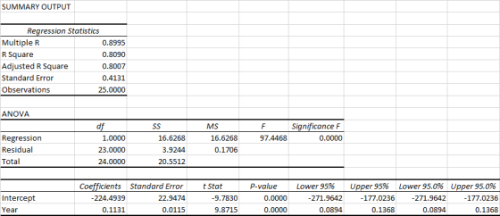
Slope coefficient for year is 0.1131, which is positive value. This indicates that there is positive relationship between year and average US gas price. Slope represents that for every one year increase, there will be 0.1131 dollars per gallon increase in the average US gas price .

Intercept value is -224.4939

Therefore, regression equation will become

Average US gas price = -224.4939 + 0.1131(year)

There is a significant relationship year and average US gas price because the p values corresponding to intercept and slope are 0.0000, which are significant.

Coefficient of determination r squared = 0.8090. This means that 80.90% of the variation in the average US gas price can be explained by the given regression equation or model.