Question

Econometrics Midterm Exam First Name: uskals Last Name: Sunculk ReddySIN: Grade: Two of the most important econometric concepts to date have been the stochastic error term and the residual. Carefully distinguish between these two concepts, being sure to: (a) Define both terms. (b) State how they are similar. (c) State how they are different. (d) Give an example of an equation that contains a stochastic error term. (e) Give an example of an equation that contains a residual. Consider the following estimated equation: C = 18.5 -0.07P, +0.93YD, -0.74D-1.3D. -1.3D, where: C -per-capita pounds of pork consumed in the United States in quartert P = the price of a hundred pounds of pork (in dollars) in quartert YD,- per capita disposable income (in dollars) in quartert D = dummy equal to 1 in the first quarter (Jan-Mar.) of the year and otherwise Dy dummy equal to 1 in the second quarter of the year and otherwise D = dummy equal to 1 in the third quarter of the year and otherwise (a) What is the meaning of the estimated coefficient of YD? (b) Specify expected signs for each of the coefficients. Explain your reasoning. (C) Suppose we changed the definition of Dso that it was equal to 1 in the fourth quarter and o otherwise and re-estimated the equation with all the other variables unchanged. Which of the estimated coefficients would change? Would your answer to part (b) above change? Explain your answer. Briefly identify the following in words or equations as appropriate: (a) p-value (b) Sampling distribution of B (e) Type 1 Error (d) Level of significance (e) Given B - 4.0 and SE (B) = 2.0, test the null hypothesis that 30 (versus the alternative hypothesis that it does not equal zero) with 13 degrees of freedom at the 1% level of significance. 4. Consider the following regression equation for the United States (standard errors in parentheses)

Answer 1

a) The error (or disturbance) of an observed value is the deviation of the observed value from the (unobservable) true value of a quantity of interest (for example, a population mean), and the residual of an observed value is the difference between the observed value and the estimated value of the quantity of interest (for example, a sample mean).

b) Residual is also a type of error but stochastic error is the difference of the observed from the true value whereas residual is from estimated value

c) The error term is the difference between the observed value for the dependent variable and its theoretical value, while a model is applied on overall population. We don't actually calculate it.

Residual is the practically calculated term during modeling exercise; It is the difference between the actual value in the sample and predicated value in the sample.

d)

In econometric theory, the classical normal linear regression model (CNLRM) involves finding the best fitting linear model for observed data that shows the relationship between two variables.

For example, let’s say you were running a study on the way the number of exams in a certain college affect the amount of red bull purchased from college vending machines. You could collect data which told you how many exams were given and how much red bull was purchased on a dozen or more days during the semester. This data can be plotted as a scatter plot, with exams (E^x) per given day on the x axis and red bull purchased (R^B) per given day on the y axis. Then you would look for the line y = β₀ + β₁ x that best fit the data.

y = 0.5297x + 28.796 + error r= 0.71 CD92 77 78 36 37 39 43 45 47 41 CD76

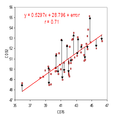
Errors on a scatter plot.

“Best fit” here means that the error term, the distance from each point to the line, is minimized. Since the relationship between variables is probably not completely linear and because there are other factors outside the scope of our study (sales on red bull, sales on other caffeine drinks, difficult physics homework sets, etc.) the graph won’t actually go through all our data points. The distance between each point and the linear graph (shown as black arrows on the above graph) is our error term. So we can write our function as R^B=β₀ + β₁ E^x + ε where β₀ and β₁ are constants and ε is an (non constant) error term.

e)

Suppose that we are given the following set of paired data:

(1, 2), (2, 3), (3, 7), (3, 6), (4, 9), (5, 9)

By using software we can see that the least squares regression line is y = 2x. We will use this to predict values for each value of x.

For example, when x = 5 we see that 2(5) = 10. This gives us the point along our regression line that has an x coordinate of 5.

To calculate the residual at the points x = 5, we subtract the predicted value from our observed value. Since the y coordinate of our data point was 9, this gives a residual of 9 – 10 = -1.

In the following table we see how to calculate all of our residuals for this data set:

X	Observed y	Predicted y	Residual
1	2	2	0
2	3	4	-1
3	7	6	1
3	6	6	0
4	9	8	1
5	9	10	-1