Question

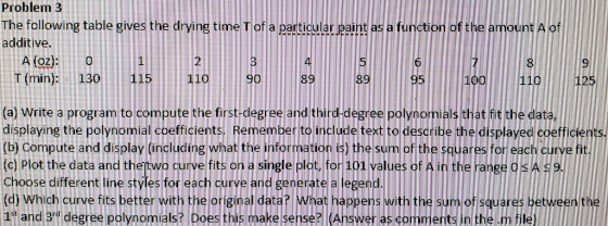
Matlab:

a) Write a program to compute the first-degree and third-degree polynomials that fit the data, displaying the polynomial coefficients. Remember to include text to describe the displayed coefficients.

(b) Compute and display (including what the information is) the sum of the squares for each curve fit.

(c) Plot the data and the two curve fits on a single plot, for 101 values of A in the range 0 ? A ? 9. Choose different line styles for each curve and generate a legend.

(d) Which curve fits better with the original data? What happens with the sum of squares between the 1^st and 3^rd degree polynomials? Does this make sense? (Answer as comments in the .m file)

Problem 3 The following table gives the drying time T of a particular paint as a function of the amount A of additive. A (oz): 2 T (min): 130 115110 9o 89 3995 (a) Write a program to compute the first-degree and third-degree polynomials that fit the data, displaying the polynomial coeficients. Remember to include text to describe the displayed coefficients. (b) compute and display tincluding what the information isi the sum of the squares for each curvt (c) Plot the data and thertwo curve fits on a single plot, for 101 values ofA in the range osAS9. Choose different line styles for each curve and generate a legend (d) Which curve fits better with the original data? What happens with the sum of squares between the 1 and 3rd degree polynomials? Does this make sense? (Answer as comments in the .m file

Answer 1

Answer:

Please find below the code for the above requirement:

A = [0,1,2,3,4,5,6,7,8,9];
A1 = linspace(0,9,101);
T = [130,115,110,90,89,89,95,100,110,125];

poly1 = polyval(polyfit(A,T,1),A1);
disp(' =First-degree polynomial coefficient: ');
disp(polyfit(A,T,1));

poly3 = polyval(polyfit(A,T,3),A1);
disp("Third-degree polynomial coefficient:")
disp(polyfit(A,T,3))

func = @(x,A)x(1)*exp(x(2)*A);

lsqcurvefit(func,A1,A,T)

plot(A,T,'o',A1,poly1,A1,poly3)

xlabel('A(oz)')
ylabel('T')
legend('Data','Linear Fit','Cubic Fit') % linear is for first order and cubic is for third order

PFB snapshot of the output:

octave:3> source ("polynomial.m") First-degree polynomial coefficient: 0.69697 108.43636 Third-degree polynomial coefficient: 1.0684e-02 1.7611e+00 -1.7352e+01 1.3103e+02 ans 1.0888e+02 7.4823e-03 1.8000e-01 2.7000e-01 3.6000e-01 4.5000e-01 5.4000e-01 6.3000e-01 7.2000e-01 8.1000e-01 9.0000e-01 9.9000e-01 1.0800e+00 1.1700e+00 1.2600e+00 1.3500e+00 1.4400e+00 1.5300e+00 1.6200e+00 1.7100e+00 1.8000e+00 1.8900e+00

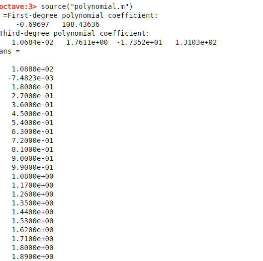
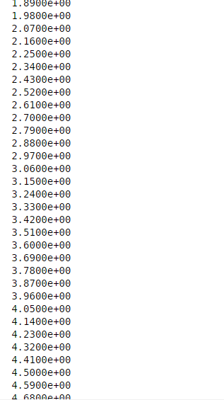
The list of values are the sum of square values:

1.9800e+00 2.0700e+00 2. 1600е+00 2. 2500е+00 2. 3400е+00 2. 4300е+00 2. 5200е+00 2. 6100е+00 2. 7000е+00 2. 7900е+00 2. 8800е 2. 9700е 3. 1500е+00 3. 2400е+00 3.3300e+00 3. 4200е+00 3. 5100е+00 3. 6900е+00 3.7800e+00 3. 8700е+00 3.9600e+00 4.0500e+00 4. 1400е+00 4.2300e+00 4. 3200е+00 4. 4100е+00 4. 5000е+00 4. 5900е+00

4. 7700е+00 4. 8600е+00 4. 9500е+00 5. 1300е+00 5. 2200е+00 5. 3100е+00 5. 4900е+00 5. 5800е+00 5. 6700е+00 5. 7600е+00 5. 8500е+00 5. 9400е+00 б. 0300е+00 6. 1200е+00 6. 2100е+00 6 . 3000е+00 6 . 3900е+00 6. 4800е+00 6. 5700е+00 6. 6600е+00 6 . 7500е+00 6. 8400е+00 6 . 9300е+00 7. 0200е+00 7. 1100е+00 7. 2000е+00 7. 2900е+00 7. 3800е+00

7.3800e+00 7. 4700е+00 7.5600e+00 7. 6500е+00 7. 7400е+00 7. 8300е+00 7. 9200е+00 8. 0100е+00 8.1000e+00 8.1900e +00 8. 2800е+00 8. 3700е+00 8.4600e+00 8. 5500е+00 8.6400e+00 8. 7300е+00 8. 8200е+00 8. 9100е+00 9. 0000е+00

Below is the output of the plot of the curves for first degree and third degree polynomials:

140 Data Linear Fit 13 120 -110 100 90 80 4 ti 10 A(oz) OZ