
Homework Answers
the response will just be the same curve with all the amplitudes multiplied with 10
the output equation will be
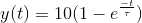
so the value of y(t) will be 6.32 at t=1 sec
Add Answer to:
If the DC gain were equal to 10 would the output curve to
10?
Also if...
II. Consider a continuous time signal x(t), containing two windowed sinusoids 0.1 0.2 0.3 0.4 0.5...
 II. Consider a continuous time signal x(t), containing two windowed sinusoids 0.1 0.2 0.3 0.4 0.5 0.6 The Fourier transform of the signal is as follows: 15 10 5 -800-_-400 h 200 400 600 The signal x(t) is the input of an LTI filter with frequency response lH(c) shown below 0.5 -&- 400︺-200 0 200 400 600 Shown below are four possible outputs of LTI filter when x(t) is the input. Please select the correct output (a) ya(t) (b) y(t)...
Create chart or table Consider the system with the impulse response ht)e u(t), as shown in Figure...
 Create chart or table Consider the system with the impulse response ht)e u(t), as shown in Figure 3.2(a). This system's response to an input of x(t) 1) would be y(t) h(r ult 1). as shown in Figure 3.2(b). If the input signal is a sum of weighted, time-shifted impulses as described by (3.10), separated in time by Δ = 0.1 (s) so that xt)01-0.1k), as shown in Figure 3.2(c), then, according to (3.11), the output is This output signal is...
intelligent control systems fuzzy logic based contril 0.8 0.7 04 0.3 0.2 0.3 b) Plot the ou a) Plot the output: -...
 intelligent control systems
fuzzy logic based contril
0.8 0.7 04 0.3 0.2 0.3 b) Plot the ou a) Plot the output: -BUB 1.0 0.9 0.9 0.8 0.7 0.6 0.5 0.4 0.3 0.5 0.4A 0.3 0.2 0.2 0.17 0.1 c) Determine the defuzzified output y, by using I. Center of Gravity Method (COG) Height Method (H) II. + 1 (0.5)+3 05)+ 5(0.1) 6()
0.8 0.7 04 0.3 0.2 0.3 b) Plot the ou a) Plot the output: -BUB 1.0 0.9 0.9...
intelligent control systems
fuzzy logic based contril
0.8 0.7 04 0.3 0.2 0.3 b) Plot the ou a) Plot the output: -BUB 1.0 0.9 0.9 0.8 0.7 0.6 0.5 0.4 0.3 0.5 0.4A 0.3 0.2 0.2 0.17 0.1 c) Determine the defuzzified output y, by using I. Center of Gravity Method (COG) Height Method (H) II. + 1 (0.5)+3 05)+ 5(0.1) 6()
0.8 0.7 04 0.3 0.2 0.3 b) Plot the ou a) Plot the output: -BUB 1.0 0.9 0.9...
The diode in the circuit below has a saturation current Is-10-13 A and n=1. Its ID-VD...
 The diode in the circuit below has a saturation current Is-10-13 A and n=1. Its ID-VD curve is illustrated below for your convenience. Problem 2 a) Using the graphical method, determine the value of R that would result in a diode current Ip -4mA. What is the resulting voltage Vp? b) With R as calculated above, a sinusoidal signal v, 100 sin(cot) mV is superimposed on the DC source. Draw the small signal model and find the output voltage across...
Thirty-two people were chosen at random from employees of a large company. Their commute times (in...
Thirty-two people were chosen at random from employees of a large company. Their commute times (in hours) were recorded in a table (shown bellow). 0.4, 0.9, 0.3, 0.5, 0.7, 1.2, 1.1, 0.7 0.6, 0.5, 0.8, 1.1, 0.9, 0.2, 0.5, 1.0 0.9, 1.0, 0.7, 0.2, 0.6, 1.1, 0.7, 1.1 0.5, 1.3, 0.7,0.6, 1.0, 0.8, 0.5, 0.9 Construct a frequency table using a class interval width of 0.2 starting at 0.15. Class Interval Frequency 0.15−0.35 0.35−0.55 0.55−0.75 0.75−0.95 0.95−1.15 ...
9. For a fuzzy system with double inputs and single output, x and y are the...
 9. For a fuzzy system with double inputs and single output, x and y are the inputs, z is the output. Assume that the elements of the inputs and output in fuzzy domains are X-fa1,a2,a3), Y={b1,b2,b3}, Z-(c1,c2,c3}, respectively. The relation between inputs and output can be described by the following fuzzy rules: Ifx is A1 and y is B1, then z is C1, where A1 and C1 B2 0.7 0.5 0.2 + a3 0.3 0.4 0.9 0.6 0.8 0.1 b1...
Using the calibration curve, calculate the molar concentration for a solution with a measured absorbance of...
 Using the calibration curve, calculate the molar concentration for
a solution with a measured absorbance of 0.143.
Concentration = M
0.7 0.6 y = 0.337x 0.5 0.4 Absorbance 0.3 0.2 0.1 o o 0.2 0.4 0.6 0.8 1 1.2 1.4 1.6 1.8 2 Concentration, M
Using the calibration curve, calculate the molar concentration for
a solution with a measured absorbance of 0.143.
Concentration = M
0.7 0.6 y = 0.337x 0.5 0.4 Absorbance 0.3 0.2 0.1 o o 0.2 0.4 0.6 0.8 1 1.2 1.4 1.6 1.8 2 Concentration, M
0.5/10 points Previous Answers MendStat14 1.E.030 My Notes Ask Your Teacher To decide on the number...
 0.5/10 points Previous Answers MendStat14 1.E.030 My Notes Ask Your Teacher To decide on the number of service centers needed for store to be built in the future, a supermarket chain wanted to obtain information on the length of time in minutes) required to service customers. To find the distribution of customer service me, a ngle of customer's 3.0 0.6 1.7 0.7 10 1.1 1.3 4.6 0.4 10 15 0.6 1.6 2.8 14 06 1.8 1.1 0.9 3.1 0.3 0.2...
B13. (Excel: Portfolio returns and stand 996 a standard deviation of 10%, and HMT has an...
 B13. (Excel: Portfolio returns and stand 996 a standard deviation of 10%, and HMT has an expected return of 12% and a standard ation of 20%. The portfolio return and risk, of course, depend on the portfolio weight ard deviations) ARC has an expected return of dev,. rtfolio returns and stan- the correlation between ARC and HMT returns. Calculate the portfolio returns and ad dard deviations for the weights and correlations shown in the table PORTFOLIO STANDARD DEVIATION WEIGHTS FOR...
Closed-loop system response and characteristics, Proportional gain 10 < paste transfer function T...
 Closed-loop system response and characteristics, Proportional gain 10 < paste transfer function Ts as output from Matlab here> clear all: close all: ls J = 0.022R = 0.11;K = 0.02;R 1.5;L= 0.6; Closed loop Transfer function T(s) Cs-10; RRA pole (Tg) 22T zero (Tg) figure ; figure ; teS) characteristics natural frequency damping ratio Dr-abs(real (RpT (2)) ) / ettling time peak time ER忌 overshoot 032=100 rise time Step response of open-loop system: Pole-zero map: easte,pole-zero plot here> Pole-Zero Map...
 II. Consider a continuous time signal x(t), containing two windowed sinusoids 0.1 0.2 0.3 0.4 0.5 0.6 The Fourier transform of the signal is as follows: 15 10 5 -800-_-400 h 200 400 600 The signal x(t) is the input of an LTI filter with frequency response lH(c) shown below 0.5 -&- 400︺-200 0 200 400 600 Shown below are four possible outputs of LTI filter when x(t) is the input. Please select the correct output (a) ya(t) (b) y(t)...
 Create chart or table Consider the system with the impulse response ht)e u(t), as shown in Figure 3.2(a). This system's response to an input of x(t) 1) would be y(t) h(r ult 1). as shown in Figure 3.2(b). If the input signal is a sum of weighted, time-shifted impulses as described by (3.10), separated in time by Δ = 0.1 (s) so that xt)01-0.1k), as shown in Figure 3.2(c), then, according to (3.11), the output is This output signal is...
 intelligent control systems
fuzzy logic based contril
0.8 0.7 04 0.3 0.2 0.3 b) Plot the ou a) Plot the output: -BUB 1.0 0.9 0.9 0.8 0.7 0.6 0.5 0.4 0.3 0.5 0.4A 0.3 0.2 0.2 0.17 0.1 c) Determine the defuzzified output y, by using I. Center of Gravity Method (COG) Height Method (H) II. + 1 (0.5)+3 05)+ 5(0.1) 6()
0.8 0.7 04 0.3 0.2 0.3 b) Plot the ou a) Plot the output: -BUB 1.0 0.9 0.9...
intelligent control systems
fuzzy logic based contril
0.8 0.7 04 0.3 0.2 0.3 b) Plot the ou a) Plot the output: -BUB 1.0 0.9 0.9 0.8 0.7 0.6 0.5 0.4 0.3 0.5 0.4A 0.3 0.2 0.2 0.17 0.1 c) Determine the defuzzified output y, by using I. Center of Gravity Method (COG) Height Method (H) II. + 1 (0.5)+3 05)+ 5(0.1) 6()
0.8 0.7 04 0.3 0.2 0.3 b) Plot the ou a) Plot the output: -BUB 1.0 0.9 0.9...
 The diode in the circuit below has a saturation current Is-10-13 A and n=1. Its ID-VD curve is illustrated below for your convenience. Problem 2 a) Using the graphical method, determine the value of R that would result in a diode current Ip -4mA. What is the resulting voltage Vp? b) With R as calculated above, a sinusoidal signal v, 100 sin(cot) mV is superimposed on the DC source. Draw the small signal model and find the output voltage across...
 9. For a fuzzy system with double inputs and single output, x and y are the inputs, z is the output. Assume that the elements of the inputs and output in fuzzy domains are X-fa1,a2,a3), Y={b1,b2,b3}, Z-(c1,c2,c3}, respectively. The relation between inputs and output can be described by the following fuzzy rules: Ifx is A1 and y is B1, then z is C1, where A1 and C1 B2 0.7 0.5 0.2 + a3 0.3 0.4 0.9 0.6 0.8 0.1 b1...
 Using the calibration curve, calculate the molar concentration for
a solution with a measured absorbance of 0.143.
Concentration = M
0.7 0.6 y = 0.337x 0.5 0.4 Absorbance 0.3 0.2 0.1 o o 0.2 0.4 0.6 0.8 1 1.2 1.4 1.6 1.8 2 Concentration, M
Using the calibration curve, calculate the molar concentration for
a solution with a measured absorbance of 0.143.
Concentration = M
0.7 0.6 y = 0.337x 0.5 0.4 Absorbance 0.3 0.2 0.1 o o 0.2 0.4 0.6 0.8 1 1.2 1.4 1.6 1.8 2 Concentration, M
 0.5/10 points Previous Answers MendStat14 1.E.030 My Notes Ask Your Teacher To decide on the number of service centers needed for store to be built in the future, a supermarket chain wanted to obtain information on the length of time in minutes) required to service customers. To find the distribution of customer service me, a ngle of customer's 3.0 0.6 1.7 0.7 10 1.1 1.3 4.6 0.4 10 15 0.6 1.6 2.8 14 06 1.8 1.1 0.9 3.1 0.3 0.2...
 B13. (Excel: Portfolio returns and stand 996 a standard deviation of 10%, and HMT has an expected return of 12% and a standard ation of 20%. The portfolio return and risk, of course, depend on the portfolio weight ard deviations) ARC has an expected return of dev,. rtfolio returns and stan- the correlation between ARC and HMT returns. Calculate the portfolio returns and ad dard deviations for the weights and correlations shown in the table PORTFOLIO STANDARD DEVIATION WEIGHTS FOR...
 Closed-loop system response and characteristics, Proportional gain 10 < paste transfer function Ts as output from Matlab here> clear all: close all: ls J = 0.022R = 0.11;K = 0.02;R 1.5;L= 0.6; Closed loop Transfer function T(s) Cs-10; RRA pole (Tg) 22T zero (Tg) figure ; figure ; teS) characteristics natural frequency damping ratio Dr-abs(real (RpT (2)) ) / ettling time peak time ER忌 overshoot 032=100 rise time Step response of open-loop system: Pole-zero map: easte,pole-zero plot here> Pole-Zero Map...
Most questions answered within 3 hours.
-
What percent of revenue does net income represent for each
year?
Total Revenue
2017 = 60,319,000...
asked 9 minutes ago -
For Ti+2 (Z=22). Determine the correct ground state
& # of microstates. Use the correct tanabe...
asked 13 minutes ago -
Why did so many investment banks have to start buying CDO’s and
other mortgaged backed securities...
asked 28 minutes ago -
The mean cost of domestic airfares in the United States rose to
an all-time high of...
asked 39 minutes ago -
1.Magazine Luiza is a Brazilian retail chain for consumer
electronics. The company currently has 100 stores...
asked 37 minutes ago -
What is the molarity of ZnCl2 that forms when 25.0 g of zinc
completely reacts with...
asked 39 minutes ago -
For independent X and Y, we have probability density function
for them where pdf of X...
asked 50 minutes ago -
The decomposition of SO2Cl2 is first order in SO2Cl2 and has a
rate constant of 1.42...
asked 46 minutes ago -
How do I convert from volume percent to mole percent in the
distillation lab? ethy acetate...
asked 53 minutes ago -
8. An air-plane has an effective wing surface area of 14.0 m²
that is generating the...
asked 54 minutes ago -
A railroad worker was a person who worked on setting and moving
railroad tracks. In securing...
asked 52 minutes ago -
using RECURSIVE Functions in Java, create a public static String
doubleLetters (String word)
For ex) that...
asked 59 minutes ago