
Homework Answers
 Copyable
Code:
Copyable
Code:
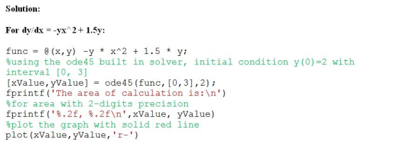
For dy/dx = -yx^2 + 1.5y:
func = @(x,y) -y * x^2 + 1.5 * y;
%using the ode45 built in solver, initial condition y(0)=2 with
interval [0, 3]
[xValue,yValue] = ode45(func,[0,3],2);
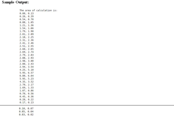
fprintf('The area of calculation is:\n')
%for area with 2-digits precision
fprintf('%.2f, %.2f\n',xValue, yValue)
%plot the graph with solid red line
plot(xValue,yValue,'r-')
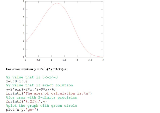
For exact solution y = 2e^-(2 x ^3-9x)/6:
%x value that is 0<=x<=3
x=0:0.1:3;
%y value that is exact solution
y=2*exp(-2*x.^3-9*x)/6;
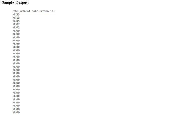
fprintf('The area of calculation is:\n')
%for area with 2-digits precision
fprintf('%.2f\n',y)
%plot the graph with green circle
plot(x,y,'go-')
Add Answer to:
Use a MATLAB built-in solver to numerically solve: dy/dx = -yx^2 + 1.5y for 0 lessthanorequalto...
Using matlab solve numerically dy/dt = sin t, y(0)=0 for 0<=t<=4π the exact solution is y(t...
using matlab solve numerically dy/dt = sin t, y(0)=0 for 0<=t<=4π the exact solution is y(t) = 1 - cos t. Compare the exact and numerical solution.
Solve the differential equation and use matlab to plot the solution 2. dy +2xy f(x), y(0) = 2 dx f(x)=x0sx<1 l...
 Solve the differential equation and use matlab to plot the solution 2. dy +2xy f(x), y(0) = 2 dx f(x)=x0sx<1 l0 x 2 1
Solve the differential equation and use matlab to plot the solution 2. dy +2xy f(x), y(0) = 2 dx f(x)=x0sx
Solve the differential equation and use matlab to plot the solution 2. dy +2xy f(x), y(0) = 2 dx f(x)=x0sx<1 l0 x 2 1
Solve the differential equation and use matlab to plot the solution 2. dy +2xy f(x), y(0) = 2 dx f(x)=x0sx
Numerical PDE Write a MatLab program to solve this equation numerically. Don't use MATLAB'S built-in functions,...
Numerical PDE Write a MatLab program to solve this equation numerically. Don't use MATLAB'S built-in functions, please. dy/dt = e ^ y − αy, y(0) = 0 where α > 0 is a parameter. Discuss the equilibrium points, the values when e^y = αy and the case when α = 0
2. Using the MATLAB "integral" command, numerically determine the Fourier Cosine series of the following function....
 2. Using the MATLAB "integral" command, numerically determine the Fourier Cosine series of the following function. Assume each case has an even extension (b,-0) Last Name N-Z: f= 2xcos (Vx+4), 0<x<3 (Hint: after extension L-3) Have your code plot both the analytical function (as a red line) and the numerical Fourier series (in blue circles -spaced appropriately). Use the Legend command to identify the two items. It is suggested to use a series with 15 terms.
Problem 1. Consider the harmonic function 2 cos 3x 1xs5 Investigate the validity of the numerical...
 Problem 1. Consider the harmonic function 2 cos 3x 1xs5 Investigate the validity of the numerical differentiation process by considering two different values for the number of points in the domain: (a) 11, and (b) 101 Plot the exact derivative of function y vs approximate (ie numerically determined) derivative of function y for both cases Qi. What is exact value of " for x=1.6? dx dy for x Q2. What is approximate value of 1.6 when number of points is...
Problem #3: The Ralston method is a second-order method that can be used to solve an...
 Problem #3: The Ralston method is a second-order method that can be used to solve an initial-value, first-order ordinary differential equation. The algorithm is given below: 2 Yi+1 = yi + k +k2)h Where kı = f(ti,y;) 3 k2 = ft;+ -h, y; +-kih You are asked to do the following: 3.1 Following that given in Inclass activity #10a, develop a MATLAB function to implement the algorithm for any given function, the time span, and the initial value. 3.2 Use...
4. Using inbuilt function in MATLAB, solve the differential equations: dx --t2 dt subject to the ...
 Matlab Code for these please.
4. Using inbuilt function in MATLAB, solve the differential equations: dx --t2 dt subject to the condition (01 integrated from0 tot 2. Compare the obtained numerical solution with exact solution 5. Lotka-Volterra predator prey model in the form of system of differential equations is as follows: dry dt dy dt where r denotes the number of prey, y refer to the number of predators, a defines the growth rate of prey population, B defines the...
Matlab Code for these please.
4. Using inbuilt function in MATLAB, solve the differential equations: dx --t2 dt subject to the condition (01 integrated from0 tot 2. Compare the obtained numerical solution with exact solution 5. Lotka-Volterra predator prey model in the form of system of differential equations is as follows: dry dt dy dt where r denotes the number of prey, y refer to the number of predators, a defines the growth rate of prey population, B defines the...
Problem #3: The Ralston method is a second-order method that can be used to solve an...
 Problem #3: The Ralston method is a second-order method that can be used to solve an initial-value, first-orde ordinary differential equation. The algorithm is given below: Vi#l=>: +($k+ş kz)h Where ky = f(ti,y:) * = f(mehr) You are asked to do the following: 3.1 Following that given in Inclass activity #10a, develop a MATLAB function to implement the algorithm for any given function, the time span, and the initial value. 3.2 Use your code to solve the following first-order ordinary...
4. * Using your calculations from 3., plot the exact solution to dy = 1-y, dt y(0) = 1/2, for 0 <ts1, along with the numerical solution given by Euler's method and the trapezoid method, both w...
 4. * Using your calculations from 3., plot the exact solution to dy = 1-y, dt y(0) = 1/2, for 0 <ts1, along with the numerical solution given by Euler's method and the trapezoid method, both with stepsize h = 0.1. Give the approximation of y(t = 1) for each numerical method. To distinguish your solutions: (i) Plot the Euler solution using crosses; do not join them with line segments. (ii) Plot the trapezoid solution using squares; again do not...
Numerical Methods Consider the following IVP dy=0.01(70-y)(50-y), with y(0)-0 (a) [10 marks Use the Runge-Kutta method of order four to obtain an approximate solution to the ODE at the points t-0.5 an...
 Numerical Methods
Consider the following IVP dy=0.01(70-y)(50-y), with y(0)-0 (a) [10 marks Use the Runge-Kutta method of order four to obtain an approximate solution to the ODE at the points t-0.5 and t1 with a step sizeh 0.5. b) [8 marks Find the exact solution analytically. (c) 7 marks] Use MATLAB to plot the graph of the true and approximate solutions in one figure over the interval [.201. Display graphically the true errors after each steps of calculations.
Consider the...
Numerical Methods
Consider the following IVP dy=0.01(70-y)(50-y), with y(0)-0 (a) [10 marks Use the Runge-Kutta method of order four to obtain an approximate solution to the ODE at the points t-0.5 and t1 with a step sizeh 0.5. b) [8 marks Find the exact solution analytically. (c) 7 marks] Use MATLAB to plot the graph of the true and approximate solutions in one figure over the interval [.201. Display graphically the true errors after each steps of calculations.
Consider the...
 Solve the differential equation and use matlab to plot the solution 2. dy +2xy f(x), y(0) = 2 dx f(x)=x0sx<1 l0 x 2 1
Solve the differential equation and use matlab to plot the solution 2. dy +2xy f(x), y(0) = 2 dx f(x)=x0sx
Solve the differential equation and use matlab to plot the solution 2. dy +2xy f(x), y(0) = 2 dx f(x)=x0sx<1 l0 x 2 1
Solve the differential equation and use matlab to plot the solution 2. dy +2xy f(x), y(0) = 2 dx f(x)=x0sx
 2. Using the MATLAB "integral" command, numerically determine the Fourier Cosine series of the following function. Assume each case has an even extension (b,-0) Last Name N-Z: f= 2xcos (Vx+4), 0<x<3 (Hint: after extension L-3) Have your code plot both the analytical function (as a red line) and the numerical Fourier series (in blue circles -spaced appropriately). Use the Legend command to identify the two items. It is suggested to use a series with 15 terms.
 Problem 1. Consider the harmonic function 2 cos 3x 1xs5 Investigate the validity of the numerical differentiation process by considering two different values for the number of points in the domain: (a) 11, and (b) 101 Plot the exact derivative of function y vs approximate (ie numerically determined) derivative of function y for both cases Qi. What is exact value of " for x=1.6? dx dy for x Q2. What is approximate value of 1.6 when number of points is...
 Problem #3: The Ralston method is a second-order method that can be used to solve an initial-value, first-order ordinary differential equation. The algorithm is given below: 2 Yi+1 = yi + k +k2)h Where kı = f(ti,y;) 3 k2 = ft;+ -h, y; +-kih You are asked to do the following: 3.1 Following that given in Inclass activity #10a, develop a MATLAB function to implement the algorithm for any given function, the time span, and the initial value. 3.2 Use...
 Matlab Code for these please.
4. Using inbuilt function in MATLAB, solve the differential equations: dx --t2 dt subject to the condition (01 integrated from0 tot 2. Compare the obtained numerical solution with exact solution 5. Lotka-Volterra predator prey model in the form of system of differential equations is as follows: dry dt dy dt where r denotes the number of prey, y refer to the number of predators, a defines the growth rate of prey population, B defines the...
Matlab Code for these please.
4. Using inbuilt function in MATLAB, solve the differential equations: dx --t2 dt subject to the condition (01 integrated from0 tot 2. Compare the obtained numerical solution with exact solution 5. Lotka-Volterra predator prey model in the form of system of differential equations is as follows: dry dt dy dt where r denotes the number of prey, y refer to the number of predators, a defines the growth rate of prey population, B defines the...
 Problem #3: The Ralston method is a second-order method that can be used to solve an initial-value, first-orde ordinary differential equation. The algorithm is given below: Vi#l=>: +($k+ş kz)h Where ky = f(ti,y:) * = f(mehr) You are asked to do the following: 3.1 Following that given in Inclass activity #10a, develop a MATLAB function to implement the algorithm for any given function, the time span, and the initial value. 3.2 Use your code to solve the following first-order ordinary...
 4. * Using your calculations from 3., plot the exact solution to dy = 1-y, dt y(0) = 1/2, for 0 <ts1, along with the numerical solution given by Euler's method and the trapezoid method, both with stepsize h = 0.1. Give the approximation of y(t = 1) for each numerical method. To distinguish your solutions: (i) Plot the Euler solution using crosses; do not join them with line segments. (ii) Plot the trapezoid solution using squares; again do not...
 Numerical Methods
Consider the following IVP dy=0.01(70-y)(50-y), with y(0)-0 (a) [10 marks Use the Runge-Kutta method of order four to obtain an approximate solution to the ODE at the points t-0.5 and t1 with a step sizeh 0.5. b) [8 marks Find the exact solution analytically. (c) 7 marks] Use MATLAB to plot the graph of the true and approximate solutions in one figure over the interval [.201. Display graphically the true errors after each steps of calculations.
Consider the...
Numerical Methods
Consider the following IVP dy=0.01(70-y)(50-y), with y(0)-0 (a) [10 marks Use the Runge-Kutta method of order four to obtain an approximate solution to the ODE at the points t-0.5 and t1 with a step sizeh 0.5. b) [8 marks Find the exact solution analytically. (c) 7 marks] Use MATLAB to plot the graph of the true and approximate solutions in one figure over the interval [.201. Display graphically the true errors after each steps of calculations.
Consider the...
Most questions answered within 3 hours.
-
WHAT IS THE EFFEKT OF ADD K2CO3 TO ( METHANOL OG WATER)?
asked 10 minutes ago -
Calculate the cell potential, the equilibrium constant, and the
free-energy change for: Ca(s)+Mn2+(aq)(1M)⇌Ca2+(aq)(1M)+Mn(s) given
the following...
asked 8 minutes ago -
Determine the pH at the equivalence (stoichiometric) point in
the titration of 48 mL of 0.28...
asked 8 minutes ago -
11. In CPM/PERT, an activity that is on the critical path
A. has equal values for...
asked 15 minutes ago -
Using C++ :
A Pascals triangle row is constructed by looking at the previous
row and...
asked 32 minutes ago -
With what speed will the fastest photoelectrons be emitted from
a surface whose threshold wavelength is...
asked 31 minutes ago -
The following slope distances and differences in elevations
between the tape ends were recorded for a...
asked 33 minutes ago -
1. Assuming random walk markets and normally distributed
returns, if a one day VaR on an...
asked 42 minutes ago -
(a) With a variable life insurance policy, the rate of return on
the investment (the death...
asked 52 minutes ago -
By applying what you know about Grignard reagents and the
mechanism by which benzoic acid is...
asked 1 hour ago -
For thermoplastics, explain the effects of increasing of each of
the following properties on a polymer’s...
asked 1 hour ago -
Make a menu for the user to use in python 3 that can search and
replace...
asked 1 hour ago