Question

Question 3 A more general form of Cauchy distribution is defined by the density function f(x; m, 7) = where m is the location parameter, is the scale parameter and they are both constants. We will create a function to simulate draws of a Cauchy(m, 7) distribution in this exercise using the inversion method.

Answer 1

a) cdf:

Let us define,

, implies

............................(i)

Thus,

inverse cdf:

Procedure to generate from Cauchy (m, )

Step 1 : Draw random samples from Uniform(0,1), here y~U(0,1)

Step 2: Use the expression in (i) , and the random sample in y(derived in Step 1), to get x.

Step 3: x is the required sample where, x~ Cauchy(m,)

b)

####let gamma =g###
myrcauchy<-function(n,m,g){
y=runif(n,0,1) ####random sample from U(0,1)###
x=m+g*tan(pi*(y-0.5))###random sample from Cauchy(m,g)###
return(x)
}

c)

z1<-myrcauchy(1000,2,1) ###testing the function###
z2<-rcauchy(1000,2,1) ###random sample from inbuilt R function###
q1<-quantile(z1,probs=seq(0.01,0.99,0.01)) #### sample (data) quantile ###
q2<-qcauchy(seq(0.01,0.99,0.01),2,1) ###theoritical quantile###
qqplot(q1,q2,main="qqplot")
qqline(q1,q2) ###qqline created to explain the plot properly###

Here, q1 === data quantile

d2== theoretical quantile

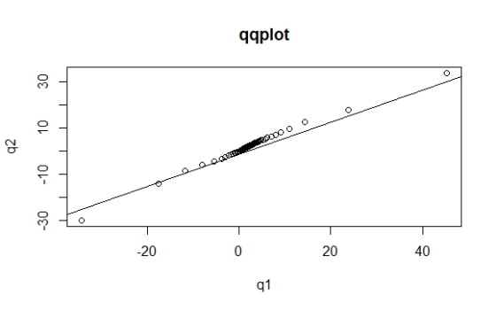
From the second diagram it can be seen that, the 45 degree line is touched by almost all the points, thus theoretical quantile and sample quantile matches.