Question

1a): Find the roots of the following polynomial equations using matlab:

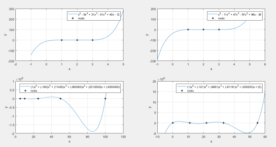
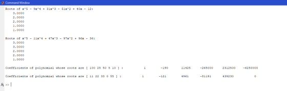
f(x) = x^5 − 9x^4 + 31x^3 − 51x^2 + 40x − 12

f(x) = x^5 − 11x^4 + 47x^3 − 97x^2 + 96x − 36

b): Find the coefficients of two polynomial equations in matlab given the following sets of roots:

r1 = [ 100 25 50 5 10 ]    r2 = [ 11 22 33 0 55 ]

c): Create a figure with four subplots, each showing a plot of one of the above functions as a line. Plot in an appropriate range to show the roots. Plot the locations of the roots as points on each subplot. Include axes labels, a legend that displays each function.

Answer 1

clear
clc

%1a
p1=[1 -9 31 -51 40 -12];
r1=roots(p1);
fprintf('Roots of x^5 - 9x^4 + 31x^3 - 51x^2 + 40x - 12:\n')
disp(r1)
p2=[1 -11 +47 -97 96 -36];
r2=roots(p2);
fprintf('Roots of x^5 - 11x^4 + 47x^3 - 97x^2 + 96x - 36: \n')
disp(r2)

%1b
r3=[100 25 50 5 10];
p3=poly(r3);
fprintf('Coefficients of polynomial whose roots are [ 100 25 50 5 10 ] :')
disp(p3)
r4=[11 22 33 0 55];
p4=poly(r4);
fprintf('Coefficients of polynomial whose roots are [ 11 22 33 0 55 ] :')
disp(p4);

%1c
subplot(2,2,1)
x=(min(r1)-2):.01:(max(r1)+2);
plot(x,polyval(p1,x),r1,polyval(p1,r1),'k*')
legend('x^5 - 9x^4 + 31x^3 - 51x^2 + 40x - 12','roots')
xlabel('x')
ylabel('y')
grid on
subplot(2,2,2)
x=(min(r2)-2):.01:(max(r2)+2);
plot(x,polyval(p2,x),r2,polyval(p2,r2),'k*')
legend('x^5 - 11x^4 + 47x^3 - 97x^2 + 96x - 36','roots')
xlabel('x')
ylabel('y')
grid on
subplot(2,2,3)
x=(min(r3)-2):.01:(max(r3)+2);
plot(x,polyval(p3,x),r3,polyval(p3,r3),'k*')
legend(sprintf('(%d)x^5 + (%d)x^4 + (%d)x^3 + (%d)x^2 + (%d)x + (%d)',p3),'roots')
xlabel('x')
ylabel('y')
grid on
subplot(2,2,4)
x=(min(r4)-5):.01:(max(r4)+5);
plot(x,polyval(p4,x),r4,polyval(p4,r4),'k*')
legend(sprintf('(%d)x^5 + (%d)x^4 + (%d)x^3 + (%d)x^2 + (%d)x + (%d)',p4),'roots')
xlabel('x')
ylabel('y')
grid on