Question

For each of the following simulation studies, please try two different sample sizes (n = 30 and n = 300). When comparing the estimators, you need to consider both of the bias and variance of the estimates across 100 simulated samples with the same sizes. Please choose your own parameter(s) for the distributions. 1. Conduct a simulation study to compare the method of moment estimator and MLE for the parameters of a Beta distribution or Gamma distribution. (You only need to pick one) 2. We established the UMVUE of p for Geometric distribution in class. Derive the UMVUE of either p2 for Geometric distribution or the UMVUE of p3 for Binomial distribution(m = 1, p)(You only need to pick one distribution. This part does not involve simulation.). Then, conduct a simulation study to compare the MLE and UMVUE 3. Conduct a simulation study to compare the power functions of the two tests (the one based on Xa) and the another one based on Σί! Xi) in the example on page 47 of the lecture note. For the test based on Σί you may also try to plot the exact power by using Gamma quantile function and Gamma cdf instead of using simulations

Answer 1

[1] 1.53479223 3.40876910 3.93477797 -1.53478242 1.83784836 -0.05523236
[7] 0.30822395 1.34377655 -1.57540597 -0.10459169 -1.06333721 -1.85164417
[13] 2.86490547 -3.36298693 0.02543367 -0.19617165 -1.02254771 1.38904882
[19] 6.58431892 -0.05340290

> mean(x)
[1] 1.083524
> sd(x)
[1] 1.736941

x<-rnorm(rep(20,each=500),1,2)

This gives us 500 means of samples of size 20 each.

> mean(x)
[1] 0.9937
> sd(x)
[1] 2.065966

This is the histogram of 500 means of samples each of size 20.

Histogram of x 髦3 髦3 12 12 し 寸 髦3 4 6 42 0

Now we make just 500 simulations

> y<-rnorm(500,1,2)

> mean(y)
[1] 1.071783
> sd(y)
[1] 1.978666

This is the histogram of 500 simulations.

Histogram of y 喾裊 収角 () 12 12 CN 0 2 4 6

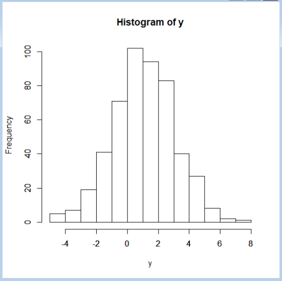
The first sample is more consistent as its the mean of the means. It's mean and sd are closer to the actual mean and sd.