
![Jsersleskandara\Desktop\New folder (7leuler.m* PUBLI.. VIEW 2 VIGATE EDIT BREAKPOINTS RUN function [xval, yval] euler (f,a,b,](http://img.homeworklib.com/images/e6ec8bad-32fd-4645-ba8b-202ae5a87c42.png?x-oss-process=image/resize,w_560)
Project 1 PDF-Summer 2019-x A 2019 La HD 16 aälall JW) x MATLAB Functions nt id 1160071 18course id 29592 1 EDE Consider the following two initial value problems along with their exact solutions FILE dy 50e-10z dr 2y, y(0) 40, re [0,2 185 -2 25 -10 y= 4 e 4 and dy cos(T) 2y, y(0) = 2, re [0,6 (6+2m2)e- y= - 2r +T sin( Tx ) +2 cos (Tz) 10 4+2 11 - 1. For each I.V.P. you should write a MATLAB script file to solve the problem ing Euler's method with the following four values of h: h 0.1, 0.01, 0.001, 0.00001 us- 2. Your code should generate a single plot of the four approximate solution curves, the exact solution and the direction field. Be sure to label the axes, the legend and the title to exactly match the information relating to each problem. a table of values including columns for r, ya, yexact corresponding only to h 0.1. The columns must be 3. In addition, please create and the absolute error labeled. printout of your code, both graphs and both tables. You will submit a *It might be easiest to embed everything into a word document for submission
Jsersleskandara\Desktop\New folder (7leuler.m* PUBLI.. VIEW 2 VIGATE EDIT BREAKPOINTS RUN function [xval, yval] euler (f,a,b, y0, h) = floor (b-a) /h +1; snumber of mesh points = (N, 1) creating an empty vector zeros (N, 1); another empty vector xval = zeros yval xval (1) = a: yval (1) y0; Efor i-2:N a+ (i-1) *h; % mesh points xval (i) (i-1) +h*f (xval (i-1), yval (i-1)) yval (i) yval sapproximate end Col 4 Ln 11 euler 14
Homework Answers

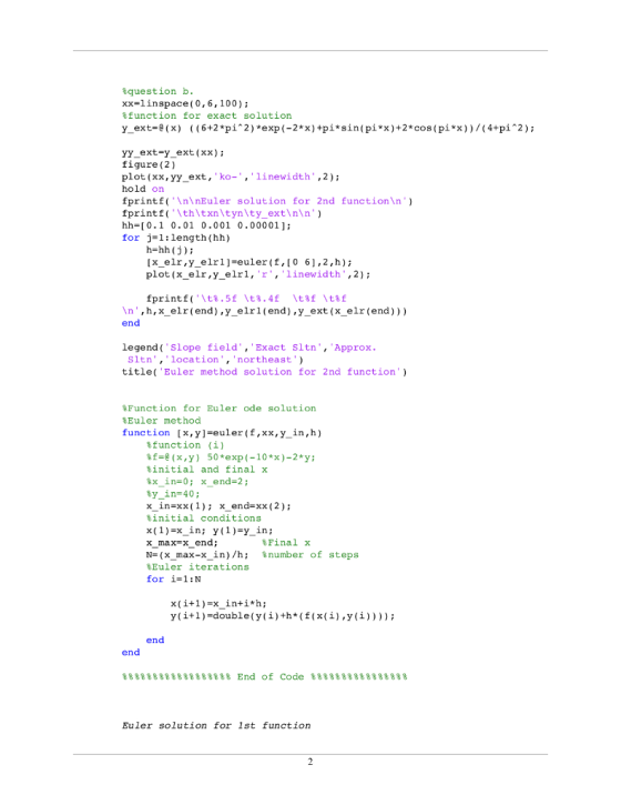
%%Matlab code for slope field of ode
clear all
close all
%function 1 for ode
f=@(x,y) 50*exp(-10*x)-2*y;
%Direction field
x=0:0.25:2; y=0:5:40;
[X,Y]=meshgrid(x,y);
dX=ones(size(X));
dY=50*exp(-10*X)-2*Y;
figure(1)
quiver(X,Y,dX,dY)
axis tight
hold on
xx=linspace(0,2,100);
%function for exact solution
y_ext=@(x) (185/4)*exp(-2*x)-(25/4)*exp(-10*x);
yy_ext=y_ext(xx);
figure(1)
plot(xx,yy_ext,'ko-','linewidth',2);
hold on
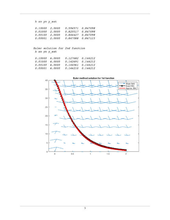
fprintf('\n\nEuler solution for 1st function\n')
fprintf('\th\txn\tyn\ty_ext\n\n')
hh=[0.1 0.01 0.001 0.00001];
for j=1:length(hh)
h=hh(j);
[x_elr,y_elr1]=euler(f,[0 2],40,h);
plot(x_elr,y_elr1,'r','linewidth',2);
fprintf('\t%.5f \t%.4f \t%f
\t%f\n',h,x_elr(end),y_elr1(end),y_ext(x_elr(end)))
end
legend('Slope field','Exact Sltn','Approx.
Sltn','location','northeast')
title('Euler method solution for 1st function')
%function 2 for ode
f=@(x,y) cos(pi*x)-2*y;
%Direction field
x=0:0.25:6; y=0:.5:3;
[X,Y]=meshgrid(x,y);
dX=ones(size(X));
dY=cos(pi*X)-2*Y;
figure(2)
quiver(X,Y,dX,dY)
axis tight
hold on
%question b.
xx=linspace(0,6,100);
%function for exact solution
y_ext=@(x)
((6+2*pi^2)*exp(-2*x)+pi*sin(pi*x)+2*cos(pi*x))/(4+pi^2);
yy_ext=y_ext(xx);
figure(2)
plot(xx,yy_ext,'ko-','linewidth',2);
hold on
fprintf('\n\nEuler solution for 2nd function\n')
fprintf('\th\txn\tyn\ty_ext\n\n')
hh=[0.1 0.01 0.001 0.00001];
for j=1:length(hh)
h=hh(j);
[x_elr,y_elr1]=euler(f,[0 6],2,h);
plot(x_elr,y_elr1,'r','linewidth',2);
fprintf('\t%.5f \t%.4f \t%f
\t%f\n',h,x_elr(end),y_elr1(end),y_ext(x_elr(end)))
end
legend('Slope field','Exact Sltn','Approx.
Sltn','location','northeast')
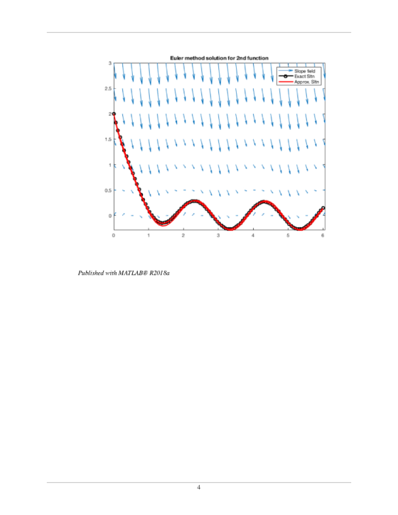
title('Euler method solution for 2nd function')
%Function for Euler ode solution
%Euler method
function [x,y]=euler(f,xx,y_in,h)
%function (i)
%f=@(x,y) 50*exp(-10*x)-2*y;
%initial and final x
%x_in=0; x_end=2;
%y_in=40;
x_in=xx(1); x_end=xx(2);
%initial conditions
x(1)=x_in;
y(1)=y_in;
x_max=x_end;
%Final x
N=(x_max-x_in)/h; %number of steps
%Euler iterations
for i=1:N
x(i+1)=x_in+i*h;
y(i+1)=double(y(i)+h*(f(x(i),y(i))));
end
end
%%%%%%%%%%%%%%%%%% End of Code %%%%%%%%%%%%%%%%
Add Answer to:
the code in the photo for this I.V.P dy/dx= x+y. y(0)=1 i need the two in the photo thank you New folder Bookmark...
3. Consider the differential equation dy 2x2y dx 0, y 1 In the following questions work...
 3. Consider the differential equation dy 2x2y dx 0, y 1 In the following questions work to 4 decimal places with the initial conditions x = throughout and give your answer to 3 decimal places, or use exact fractions (a) Use the Euler method to calculate an estimate of the value of y after four steps of length h 0.5 [4 marks] (b) Use the Modified Euler method to calculate an estimate of the value of y after two steps...
4. * Using your calculations from 3., plot the exact solution to dy = 1-y, dt y(0) = 1/2, for 0 <ts1, along with the numerical solution given by Euler's method and the trapezoid method, both w...
 4. * Using your calculations from 3., plot the exact solution to dy = 1-y, dt y(0) = 1/2, for 0 <ts1, along with the numerical solution given by Euler's method and the trapezoid method, both with stepsize h = 0.1. Give the approximation of y(t = 1) for each numerical method. To distinguish your solutions: (i) Plot the Euler solution using crosses; do not join them with line segments. (ii) Plot the trapezoid solution using squares; again do not...
For the following differential equation: (x^3)dy/dx+y^4+3=0 where dy/dx is the first derivative of y with respect...
 For the following differential equation: (x^3)dy/dx+y^4+3=0 where dy/dx is the first derivative of y with respect to x, () means power. The equation has initial values y=2.00 at x=1.00 Using Euler method with a step in the x direction of h=0.30: Show the equation to use to generate values of (2 marks) Calculate the missing values of y in the table below I .1.30 1.00 2.00 1.60 For (2 marks)
Consider the differential equation dy/dx = (y-1)/x.
 Consider the differential equation dy/dx = (y-1)/x. (a) On the axes provided, sketch a slope field for the given differential equation at the nine points indicated. (b) Let y = f (x) be the particular solution to the given differential equation with the initial condition f (3) = 2. Write an equation for the line tangent to the graph of y= f (x) at x = 3. Use the equation to approximate the value of f (3.3). (c) Find the particular solution y...
1 st s2, y(1)1 The exact solution is given by yo) - = . 1+Int Write a MATLAB code to approximate ...
 1 st s2, y(1)1 The exact solution is given by yo) - = . 1+Int Write a MATLAB code to approximate the solution of the IVP using Midpoint (RK2) and Modified Euler methods when h [0.5 0.1 0.0s 0.01 0.005 0.001]. A) Find the vector w mid and w mod that approximates the solution of the IVP for different values of h. B) Plot the step-size h versus the relative error of both in the same figure using the LOGLOG...
Question 1: Given the initial-value problem 12-21 0 <1 <1, y(0) = 1, 12+10 with exact...
 Question 1: Given the initial-value problem 12-21 0 <1 <1, y(0) = 1, 12+10 with exact solution v(t) = 2t +1 t2 + 1 a. Use Euler's method with h = 0.1 to approximate the solution of y b. Calculate the error bound and compare the actual error at each step to the error bound. c. Use the answers generated in part (a) and linear interpolation to approximate the following values of y, and compare them to the actual value...
Problem Thre: 125 points) Consider the following initial value problem: dy-2y+ t The y(0) -1 ea dt ical solution of the differential equation is: y(O)(2-2t+3e-2+1)y fr exoc the differential equat...
 Problem Thre: 125 points) Consider the following initial value problem: dy-2y+ t The y(0) -1 ea dt ical solution of the differential equation is: y(O)(2-2t+3e-2+1)y fr exoc the differential equation numerically over the interval 0 s i s 2.0 and a step size h At 0.5.A Apply the following Runge-Kutta methods for each of the step. (show your calculations) i. [0.0 0.5: Euler method ii. [0.5 1.0]: Heun method. ii. [1.0 1.5): Midpoint method. iv. [1.5 2.0): 4h RK method...
Given the initial-value problem y'=2-2tyt2+1, 0 ≤t≤1, y0=1 With exact solution yt= 2t+1t2+1 Using MATLAB use...
Given the initial-value problem y'=2-2tyt2+1, 0 ≤t≤1, y0=1 With exact solution yt= 2t+1t2+1 Using MATLAB use Euler’s method with h = 0.1 to approximate the solution of y
Q1: Solve the ODE: f) Vyy' + y3/2-1. y(1) = 0. g) (2x +y)dx(2x+y-1)dy 0. i) dx=xy2e": y(2)=0. j) ...
 Q1: Solve the ODE: f) Vyy' + y3/2-1. y(1) = 0. g) (2x +y)dx(2x+y-1)dy 0. i) dx=xy2e": y(2)=0. j) (1 + x*)dy + (1 + y*)dx = 0; y(1) = V3.
Q1: Solve the ODE: f) Vyy' + y3/2-1. y(1) = 0. g) (2x +y)dx(2x+y-1)dy 0. i) dx=xy2e": y(2)=0. j) (1 + x*)dy + (1 + y*)dx = 0; y(1) = V3.
Q1: Solve the ODE: f) Vyy' + y3/2-1. y(1) = 0. g) (2x +y)dx(2x+y-1)dy 0. i) dx=xy2e": y(2)=0. j) (1 + x*)dy + (1 + y*)dx = 0; y(1) = V3.
Matlab & Differential Equations Help Needed I need help with this Matlab project for differential equations. I've got 0 experience with Matlab other than a much easier project I did in another...
 Matlab & Differential Equations Help Needed
I need help with this Matlab project for differential equations.
I've got 0 experience with Matlab other than a much easier project
I did in another class a few semesters ago. All we've been given is
this piece of paper and some sample code. I don't even know how to
begin to approach this. I don't know how to use Matlab at all and I
barely can do this material.
Here's the handout:
Here's...
Matlab & Differential Equations Help Needed
I need help with this Matlab project for differential equations.
I've got 0 experience with Matlab other than a much easier project
I did in another class a few semesters ago. All we've been given is
this piece of paper and some sample code. I don't even know how to
begin to approach this. I don't know how to use Matlab at all and I
barely can do this material.
Here's the handout:
Here's...
 3. Consider the differential equation dy 2x2y dx 0, y 1 In the following questions work to 4 decimal places with the initial conditions x = throughout and give your answer to 3 decimal places, or use exact fractions (a) Use the Euler method to calculate an estimate of the value of y after four steps of length h 0.5 [4 marks] (b) Use the Modified Euler method to calculate an estimate of the value of y after two steps...
 4. * Using your calculations from 3., plot the exact solution to dy = 1-y, dt y(0) = 1/2, for 0 <ts1, along with the numerical solution given by Euler's method and the trapezoid method, both with stepsize h = 0.1. Give the approximation of y(t = 1) for each numerical method. To distinguish your solutions: (i) Plot the Euler solution using crosses; do not join them with line segments. (ii) Plot the trapezoid solution using squares; again do not...
 For the following differential equation: (x^3)dy/dx+y^4+3=0 where dy/dx is the first derivative of y with respect to x, () means power. The equation has initial values y=2.00 at x=1.00 Using Euler method with a step in the x direction of h=0.30: Show the equation to use to generate values of (2 marks) Calculate the missing values of y in the table below I .1.30 1.00 2.00 1.60 For (2 marks)
 1 st s2, y(1)1 The exact solution is given by yo) - = . 1+Int Write a MATLAB code to approximate the solution of the IVP using Midpoint (RK2) and Modified Euler methods when h [0.5 0.1 0.0s 0.01 0.005 0.001]. A) Find the vector w mid and w mod that approximates the solution of the IVP for different values of h. B) Plot the step-size h versus the relative error of both in the same figure using the LOGLOG...
 Question 1: Given the initial-value problem 12-21 0 <1 <1, y(0) = 1, 12+10 with exact solution v(t) = 2t +1 t2 + 1 a. Use Euler's method with h = 0.1 to approximate the solution of y b. Calculate the error bound and compare the actual error at each step to the error bound. c. Use the answers generated in part (a) and linear interpolation to approximate the following values of y, and compare them to the actual value...
 Problem Thre: 125 points) Consider the following initial value problem: dy-2y+ t The y(0) -1 ea dt ical solution of the differential equation is: y(O)(2-2t+3e-2+1)y fr exoc the differential equation numerically over the interval 0 s i s 2.0 and a step size h At 0.5.A Apply the following Runge-Kutta methods for each of the step. (show your calculations) i. [0.0 0.5: Euler method ii. [0.5 1.0]: Heun method. ii. [1.0 1.5): Midpoint method. iv. [1.5 2.0): 4h RK method...
 Q1: Solve the ODE: f) Vyy' + y3/2-1. y(1) = 0. g) (2x +y)dx(2x+y-1)dy 0. i) dx=xy2e": y(2)=0. j) (1 + x*)dy + (1 + y*)dx = 0; y(1) = V3.
Q1: Solve the ODE: f) Vyy' + y3/2-1. y(1) = 0. g) (2x +y)dx(2x+y-1)dy 0. i) dx=xy2e": y(2)=0. j) (1 + x*)dy + (1 + y*)dx = 0; y(1) = V3.
Q1: Solve the ODE: f) Vyy' + y3/2-1. y(1) = 0. g) (2x +y)dx(2x+y-1)dy 0. i) dx=xy2e": y(2)=0. j) (1 + x*)dy + (1 + y*)dx = 0; y(1) = V3.
 Matlab & Differential Equations Help Needed
I need help with this Matlab project for differential equations.
I've got 0 experience with Matlab other than a much easier project
I did in another class a few semesters ago. All we've been given is
this piece of paper and some sample code. I don't even know how to
begin to approach this. I don't know how to use Matlab at all and I
barely can do this material.
Here's the handout:
Here's...
Matlab & Differential Equations Help Needed
I need help with this Matlab project for differential equations.
I've got 0 experience with Matlab other than a much easier project
I did in another class a few semesters ago. All we've been given is
this piece of paper and some sample code. I don't even know how to
begin to approach this. I don't know how to use Matlab at all and I
barely can do this material.
Here's the handout:
Here's...
Most questions answered within 3 hours.
-
Write a program to solve the Josephus problem, with the following
modification:
Sample Input:
./a.out n...
asked 2 hours ago -
At the start of a CD it is spinning at a rate of 525 rpm
(revolutions...
asked 2 hours ago -
4. Without doing any calculations, predict whether the observed
∆T would increase, decrease or remain the...
asked 4 hours ago -
Based on the range, which of the following sets of scores has
the greatest variability? 3,...
asked 5 hours ago -
Ripples in a pond travel at a velocity of 3 m/s with one peak
passing a...
asked 5 hours ago -
A man stands on the roof of a building of height 13.0 mm and
throws a...
asked 5 hours ago -
The extent to which assets are financed by borrowed funds and
other liabilities is indicated by:...
asked 6 hours ago -
Explain in detail
Germany is the fifth largest economy
explain what goods and services Germany specializes...
asked 6 hours ago -
The density of platinum is 21.45 g/mL. If a cube of platinum
with a mass of...
asked 6 hours ago -
Accounts Receivable
Sales
A/R Posting
Extended Sales Invoice
Packing Slip
Compare invoice to packing slip 2...
asked 6 hours ago -
Michaella, age 23, is a full-time law student and is claimed by
her parents as a...
asked 6 hours ago -
Why are polymers not typically casted into products?
asked 6 hours ago