Question

Please show in excel with formulas

1. Suppose that at the end of December 2008 you purchased Inc. (Nasdaq: AAPL). It is now five years later and you decide tApple, your holdings to see if you have done well with this inv below shows the end-of-year market prices of AAP table AAPL Stock Prices Date 2008 2009 203.76 2010 311.89 2011 391.60 2012 519.13 2013 561.02 Price 82.53 Enter the data, as shown, into a worksheet and format the table as shown. Create a formula to calculate your rate of return for each year. Format the results as percentages with two decimal places. Calculate the total return for the entire five-year holding period. What is the compound average annual rate of return? a. b. c.

Answer 1

a.

b.

Formula to calculate yearly returns is:

$Yearly\:return=\frac{Price\: in \:current\: year-Price\: in \:previous\: year}{Price\: in \:previous\: year}*100$

The excel implementation is as shown:

This formula is then copied to calculate returns for all years. The completed table is as shown:

c.

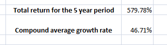
Total return can be calculated using the formula:

$Total\:return=\frac{Price\: in \:2013-Price\: in \:2008}{Price\: in \:2008}*100$

whereas the compounded average growth can be calculated using the formula:

$CAGR=\left ( \frac{Price\: in \:2013}{Price\: in \:2008} \right )^{\frac{1}{n}}-1$

n in the above formula is no. of periods which is five in the given case:

Excel implementation is as shown:

Total return calculation:

12 13 14 AAPL Stock Prices Total return for the 5 year period (C21-C16)/c1 Yearly rate of return Date Price Compound average growth rate 46.71% 15 16 17 18 19 20 21 2008 2009 203.76 2010 2011 2012 2013 82.53 311.89 391.60 519.13 561.02 146.89% 53.07% 25.56% 32.57% 8.07%

CAGR calculation:

The answers are:

d.

Charts can simply be inserted in excel by selecting the data and then going to Insert->Line/Scatter. for this case, line chart makes more sense.

e.

The charts can be customized by first selecting the chart and then going to the design option on the excel ribbon. There are many different options such as background color, 3D etc that can be chosen.