Question

R programming:

Problem One. a) Create a histogram for the attribute "Weight" and test the claim that the average car Weight is 3100 lbs. Recode the variable ET using V-Shape instead of "0" and Straight instead of"1). "save it as ETnew". Create a barplot for the new ET variable and test the claim that the proportion of a V-shaped type of engine is 0.50 Fin b) c) d a 95% confidence interval for the average car weight Find a 90% confidence interval for the proportion of a V-shaped type of engine d)

MPG   GPM   WT   DIS   NC   HP   ACC   ET
16.9   5.917   4.360   350   8   155   14.9   1
15.5   6.452   4.054   351   8   142   14.3   1
19.2   5.208   3.605   267   8   125   15.0   1
18.5   5.405   3.940   360   8   150   13.0   1
30.0   3.333   2.155   98   4   68   16.5   0
27.5   3.636   2.560   134   4   95   14.2   0
27.2   3.676   2.300   119   4   97   14.7   0
30.9   3.236   2.230   105   4   75   14.5   0
20.3   4.926   2.830   131   5   103   15.9   0
17.0   5.882   3.140   163   6   125   13.6   0
21.6   4.630   2.795   121   4   115   15.7   0
16.2   6.173   3.410   163   6   133   15.8   0
20.6   4.854   3.380   231   6   105   15.8   0
20.8   4.808   3.070   200   6   85   16.7   0
18.6   5.376   3.620   225   6   110   18.7   0
18.1   5.525   3.410   258   6   120   15.1   0
17.0   5.882   3.840   305   8   130   15.4   1
17.6   5.682   3.725   302   8   129   13.4   1
16.5   6.061   3.955   351   8   138   13.2   1
18.2   5.495   3.830   318   8   135   15.2   1
26.5   3.774   2.585   140   4   88   14.4   0
21.9   4.566   2.910   171   6   109   16.6   1
34.1   2.933   1.975   86   4   65   15.2   0
35.1   2.849   1.915   98   4   80   14.4   0
27.4   3.650   2.670   121   4   80   15.0   0
31.5   3.175   1.990   89   4   71   14.9   0
29.5   3.390   2.135   98   4   68   16.6   0
28.4   3.521   2.670   151   4   90   16.0   0
28.8   3.472   2.595   173   6   115   11.3   1
26.8   3.731   2.700   173   6   115   12.9   1
33.5   2.985   2.556   151   4   90   13.2   0
34.2   2.924   2.200   105   4   70   13.2   0
31.8   3.145   2.020   85   4   65   19.2   0
37.3   2.681   2.130   91   4   69   14.7   0
30.5   3.279   2.190   97   4   78   14.1   0
22.0   4.545   2.815   146   6   97   14.5   0
21.5   4.651   2.600   121   4   110   12.8   0
31.9   3.135   1.925   89   4   71   14.0   0

Answer 1

## ####
## For a) and c)

WT=c(4.360,4.054,3.605,3.940,2.155,2.560,2.300,2.230,2.830,3.140,2.795,
3.410,3.380,3.070,3.620,3.410,3.840,3.725,3.955,3.830,2.585,2.910,1.975,
1.915,2.670,1.990,2.135,2.670,2.595,2.700,2.556,2.200,2.020,2.130,2.190,
2.815,2.600, 1.925)

## Histogram
hist(WT)

t.test(x=WT, y = NULL,
alternative = c("two.sided"),
mu = 3.100,,
conf.level = 0.95)

#######################
### For b) and d)

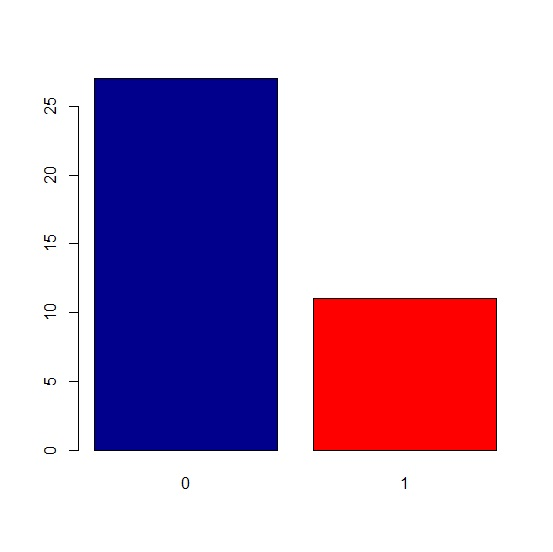
ET=c(1,1,1,1,0,0,0,0,0,0,0,0,0,0,0,0,1,1,1,1,0,1,0,0,0,0,0,0,1,1,0,0,0,0,0,
0,0,0)
n=length(ET)
ET_Sum=sum(ET)

count <- table(ET)
barplot(count, col=c("darkblue","red"))

prop.test(x=ET_Sum, n, p = 0.5,
alternative = c("two.sided"),
conf.level = 0.90)

####### Our put of the program is

> ## ####
> ## For a) and c)
>
> WT=c(4.360,4.054,3.605,3.940,2.155,2.560,2.300,2.230,2.830,3.140,2.795,
+ 3.410,3.380,3.070,3.620,3.410,3.840,3.725,3.955,3.830,2.585,2.910,1.975,
+ 1.915,2.670,1.990,2.135,2.670,2.595,2.700,2.556,2.200,2.020,2.130,2.190,
+ 2.815,2.600, 1.925)
>
> ## Histogram
> hist(WT)
>
> t.test(x=WT, y = NULL,
+ alternative = c("two.sided"),
+ mu = 3.100,,
+ conf.level = 0.95)

One Sample t-test

data: WT
t = -2.0677, df = 37, p-value = 0.04571
alternative hypothesis: true mean is not equal to 3.1
95 percent confidence interval:
2.630552 3.095237
sample estimates:
mean of x
2.862895

>
>
>
> #######################
> ### For b) and d)
>
> ET=c(1,1,1,1,0,0,0,0,0,0,0,0,0,0,0,0,1,1,1,1,0,1,0,0,0,0,0,0,1,1,0,0,0,0,0,
+ 0,0,0)
> n=length(ET)
> ET_Sum=sum(ET)
>
>
> count <- table(ET)
> barplot(count, col=c("darkblue","red"))
>
> prop.test(x=ET_Sum, n, p = 0.5,
+ alternative = c("two.sided"),
+ conf.level = 0.90)

1-sample proportions test with continuity correction

data: ET_Sum out of n, null probability 0.5
X-squared = 5.9211, df = 1, p-value = 0.01496
alternative hypothesis: true p is not equal to 0.5
90 percent confidence interval:
0.1749422 0.4349116
sample estimates:
p
0.2894737

### Histogram of a)

## Barplot of b is

10 15 20 25