Question

Parta): 1. Using the following table of relation between X & Y (Y is the independent Variable): Xi0 234 36 7 8 9 | 11 55 28 5 20 30 a. Find the estimated regression equation Show ALL your calculations and the appropriate formula. WRITE Formula in all the questions below and substitute for the numbers, demonstrate your work. As you see, some cells are blank; you are to put your student ID digits on those cells b. Calculate R2 Comment on the Goodness of the Fit. Is it a good fit? Why? c. Test the hypothesis regarding the significance of the slope Bi. (Use a = 0.05) Show ALL the calculations necessary to get your answer. Hint: You need to calculate t by using all the formulas needed for it using t in the Formula Sheet d. Calculate the values of F, using formula for F statistics. (Here, you only CALCULATING the F-Value, using the formula and are not being asked to comment on its significance). e. Draw the scatter diagram and also your estimated regression line. Part B): Perform the Simple Regression in Excel and Submit the Summary Output along with your response. Be sure the values for all the calculated values by you matches those of your Excel Print out.

Answer 1

५१ ५: 2 : (1-22 | | 255 4 | 5 | 25 20 | 3 | 246 | 6 | 86448 | | 5 | 25 35 | 8 | 20 400 160 | 30. | 900 210 . 21.7777 म.| 2.1111 .4444 2,1111 11 5.५५५५ |||||| ___18.11118. 42 11 1445 556 +2 | - = Er : 42 - 4.6666 । ५ = 2 - 2 : 8.5555 | | S५ - ५१()1५५5 - 2 5 - 186.22 __5x4 - 2845 - मादृपः - 556 - (42) (47) Sxy = 126.68

Bra Say - 196.68 - 344 786:22. | 4, 0,25011 Bo = - B. T -4.6666-0.250168.5555) = 2.5266) @ Estimated pregression equation becomes = 2053 +0.2541 SSF | 550 = ß, 3x4 - 0.2501X 196:68. 55R2 49.1896]

557= 2.C..; - 70 199, 22 R² = SSR - 49.1895 555 of 2 --- 0.6832 R2-0.6832 conclusion on 680 10 of variation in x is explained by y variable therefore | given model is good fit. @ Given ő cs 0,05 | HoBize Nis Het BEO Test statistic Ito a B, secß.) a tn 2,212 se cp d = Moren 344 0 - 2 But Msres - SSResis-384-35R D-2____ a 72- 49.1896 - 9-2

MS Res=3.258. I secß d = 3.258 V 786.22 seca) - 0.06437 to-0.2501 0.06437 to = 3.88542 t«t2, -2 = to.osg-2-50.025,7 - 2.3646 -و مهمهعمهع Here I tolyt. _then we reject Her Then we conclude that given regression coefficient (Bij is significant SSR MSR Mopeni S.SResi/n-2 49.1896 3.258 15.0980. LF151
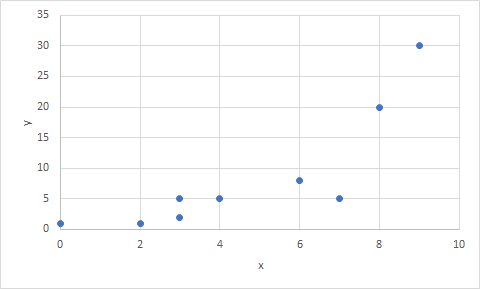
e) Scatter plot

$1585673863427_image.png$

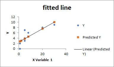
Regression fitted line

fitted line ONE Predicted Y - 40 - Linear (Predicted Y) X Variable 1

PART B)

SUMMARY OUTPUT
Regression Statistics
Multiple R	0.826593
R Square	0.683256
Adjusted R Square	0.638007
Standard Error	1.804975
Observations	9
ANOVA
	df	SS	MS	F	Significance F
Regression	1	49.19446	49.19446	15.09989	0.006007
Residual	7	22.80554	3.257934
Total	8	72
	Coefficients	Standard Error	t Stat	P-value	Lower 95%	Upper 95%	Lower 95.0%	Upper 95.0%
Intercept	2.526569	0.815664	3.097562	0.017382	0.59783	4.455307	0.59783	4.455307
X Variable 1	0.250141	0.064372	3.885858	0.006007	0.097925	0.402357	0.097925	0.402357
RESIDUAL OUTPUT
Observation	Predicted Y	Residuals
1	2.77671	-2.77671
2	2.77671	-0.77671
3	3.777275	-0.77728
4	3.777275	0.222725
5	3.026851	-0.02685
6	4.527699	1.472301
7	3.777275	3.222725
8	7.529395	0.470605
9	10.03081	-1.03081