Please to (B) in depth as its for exam review. It'd be nice to see al equations you used.

Homework Answers


Matlab Code:
syms s
s=tf('s')
x=(s+3)/(s*(s+1)*(s+5)*(s+10))
rlocus(x)
Add Answer to:
Please to (B) in depth as its for exam review. It'd be nice to
see al...
Please answer BOTH mathematicaly on paper, and with matlab( as it says in the question). Thank...
 Please answer BOTH mathematicaly on paper, and with matlab( as
it says in the question). Thank you
For each of the following loop transfer function F(s), find the portion of the root locus on the real axis, asymptotes, the arrival and departure angles at any complex zero or pole, and the frequency of any imaginary-axis crossing. Sketch the root locus based on above findings. Verify your results using Matlab. Submit plots of your hand sketches and the Matlab results. a....
Please answer BOTH mathematicaly on paper, and with matlab( as
it says in the question). Thank you
For each of the following loop transfer function F(s), find the portion of the root locus on the real axis, asymptotes, the arrival and departure angles at any complex zero or pole, and the frequency of any imaginary-axis crossing. Sketch the root locus based on above findings. Verify your results using Matlab. Submit plots of your hand sketches and the Matlab results. a....
Lectures 15-18: Root-locus method 5.1 Sketch the root locus for a unity feedback system with the ...
 help on #5.2
L(s) is loop transfer function
1+L(s) = 0
lecture notes:
Lectures 15-18: Root-locus method 5.1 Sketch the root locus for a unity feedback system with the loop transfer function (8+5(+10) .2 +10+20 where K, T, and a are nonnegative parameters. For each case summarize your results in a table similar to the one provided below. Root locus parameters Open loop poles Open loop zeros Number of zeros at infinity Number of branches Number of asymptotes Center of...
help on #5.2
L(s) is loop transfer function
1+L(s) = 0
lecture notes:
Lectures 15-18: Root-locus method 5.1 Sketch the root locus for a unity feedback system with the loop transfer function (8+5(+10) .2 +10+20 where K, T, and a are nonnegative parameters. For each case summarize your results in a table similar to the one provided below. Root locus parameters Open loop poles Open loop zeros Number of zeros at infinity Number of branches Number of asymptotes Center of...
Theroot-locus design method (d) Gos)H(s)2) 5.5 Complex poles and zeros. For the systems with an open-loop transfer function given below, sketch the root locus plot. Find the asymptotes and their angle...
 Theroot-locus design method
(d) Gos)H(s)2) 5.5 Complex poles and zeros. For the systems with an open-loop transfer function given below, sketch the root locus plot. Find the asymptotes and their angles. the break-away or break-in points, the angle of arrival or departure for the complex poles and zeros, respectively, and the range of k for closed-loop stability 5 10ん k(s+21
(d) Gos)H(s)2) 5.5 Complex poles and zeros. For the systems with an open-loop transfer function given below, sketch the root...
Theroot-locus design method
(d) Gos)H(s)2) 5.5 Complex poles and zeros. For the systems with an open-loop transfer function given below, sketch the root locus plot. Find the asymptotes and their angles. the break-away or break-in points, the angle of arrival or departure for the complex poles and zeros, respectively, and the range of k for closed-loop stability 5 10ん k(s+21
(d) Gos)H(s)2) 5.5 Complex poles and zeros. For the systems with an open-loop transfer function given below, sketch the root...
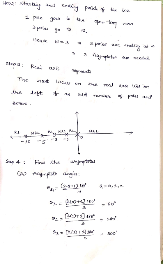
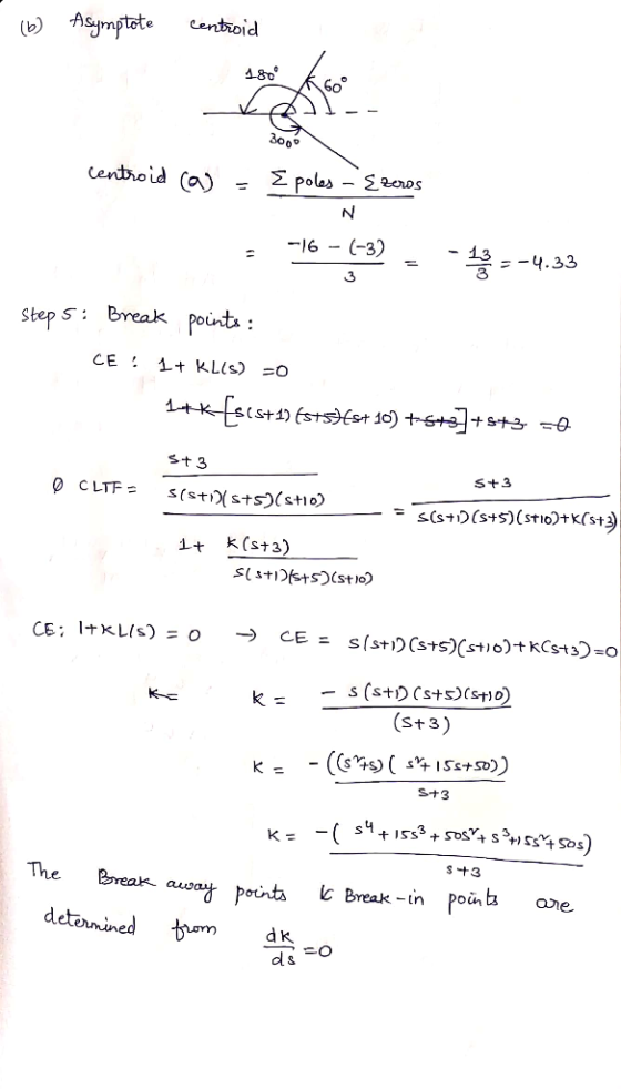
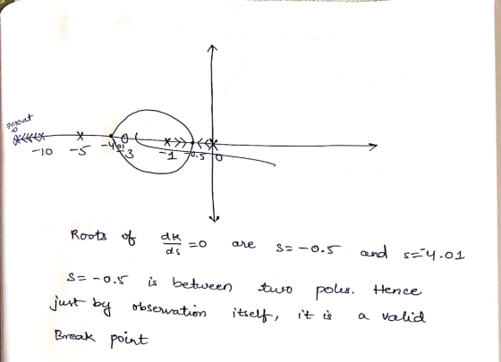
Hand sketch the root locus with respect to K for the equation 1+KL(s) = 0 where L(s) is shown below.
 Hand sketch the root locus with respect to K for the equation 1+KL(s) = 0 where L(s) is shown below. Your sketch should clearly indicate the locations of the poles (X) and the zeros (0) of the L(s). If necessary, show the location and angle of the asymptotes, location of the break-in/breakaway points, and the location at which the root locus intersects imaginary axis. After completing each hand sketch, verify your results using MATLAB. You do not submit to submit the...
The characteristic equation (denominator of the closed-loop transfer function set equal to zero) is given s3 + 2s2 + (20K +7)s+ 100K Sketch the root locus of the given system above with respect to...
 The characteristic equation (denominator of the closed-loop transfer function set equal to zero) is given s3 + 2s2 + (20K +7)s+ 100K Sketch the root locus of the given system above with respect to K. [ Find the asymptotes and their angles, the break-away or break-in points, the angle of arrival or departure for the complex poles and zeros, imaginary axis crossing points, respectively (if any).
The characteristic equation (denominator of the closed-loop transfer function set equal to zero) is...
The characteristic equation (denominator of the closed-loop transfer function set equal to zero) is given s3 + 2s2 + (20K +7)s+ 100K Sketch the root locus of the given system above with respect to K. [ Find the asymptotes and their angles, the break-away or break-in points, the angle of arrival or departure for the complex poles and zeros, imaginary axis crossing points, respectively (if any).
The characteristic equation (denominator of the closed-loop transfer function set equal to zero) is...
For the following system, R(s) Y(s) s(s +4) a)Sketch its root locus. Be sure to calculate...
 For the following system, R(s) Y(s) s(s +4) a)Sketch its root locus. Be sure to calculate (and clearly label) all asymptotes, break- away/break-in points, departure/arrival angles, and imaginary axis crossings (if any) Include arrows showing the direction of closed-loop pole traversal. b) Find the smallest time constant the system will have.
Consider proportional feedback control as shown below. r(t) For each G(s) in the following problems A....
 Consider proportional feedback control as shown below. r(t) For each G(s) in the following problems A. Sketch the root locus. Clearly show the open-loop poles and zeros, and the high-gain asymptotes on your sketch. Calculate the centroid to assure that the high gain asymptotes are accurate. B. If your sketch reveals any break-in or break-away points, calculate those location C. Does your sketch reveal a jo- crossing? If so, stability may be an issue. D. A damping ratio of 7-...
these are useful formjlas to solve this problem please show all work! thank you 2.) Design...
 these are useful formjlas to solve this problem
please show all work! thank you
2.) Design compensator for zero steady-state error with 10% overshoot and 0.4s of Peak time for the open loop transfer function G specified below. Sketch the comparison between uncompensated and compensated responses. Also compare their root locus. Clearly mention the improvements achieved after compensation. (50 points = 10 pts for analyzing uncompensated system+5 pts for identifying controller type+25 pts for controller design+5 pts for response comparison+5...
these are useful formjlas to solve this problem
please show all work! thank you
2.) Design compensator for zero steady-state error with 10% overshoot and 0.4s of Peak time for the open loop transfer function G specified below. Sketch the comparison between uncompensated and compensated responses. Also compare their root locus. Clearly mention the improvements achieved after compensation. (50 points = 10 pts for analyzing uncompensated system+5 pts for identifying controller type+25 pts for controller design+5 pts for response comparison+5...
4.) (a) Sketch the positive root locus of the system shown below using the (2, 2) Pade approximat...
 4.) (a) Sketch the positive root locus of the system shown below using the (2, 2) Pade approximation for the delay. State the asymptote angles and their centroid, the arrival and departure angles at any complex pole or zero, the frequencies of any imaginary axis crossings, and the locations of any break-in or break-away points. (b) Use Matlab to plot the positive root locus of the system shown below using the (2, 2) Pade approximation for the delay. Your sketch...
oble2 (25 Pts.) Root Locus: A proportional only action is controlling a plant with unity feedback. The plant ansfer function is: 6 GG)s+ 1)s + 2)s +3) a. Draw the poles of G(s) in below figure b....
 oble2 (25 Pts.) Root Locus: A proportional only action is controlling a plant with unity feedback. The plant ansfer function is: 6 GG)s+ 1)s + 2)s +3) a. Draw the poles of G(s) in below figure b. How many asymptotes does the root locus plot of the above transfer function has? c. What angles do the asymptotes make with the positive real axis in the s plane? d. At what point do the asymptotes intersect on the real axis? e....
 Please answer BOTH mathematicaly on paper, and with matlab( as
it says in the question). Thank you
For each of the following loop transfer function F(s), find the portion of the root locus on the real axis, asymptotes, the arrival and departure angles at any complex zero or pole, and the frequency of any imaginary-axis crossing. Sketch the root locus based on above findings. Verify your results using Matlab. Submit plots of your hand sketches and the Matlab results. a....
Please answer BOTH mathematicaly on paper, and with matlab( as
it says in the question). Thank you
For each of the following loop transfer function F(s), find the portion of the root locus on the real axis, asymptotes, the arrival and departure angles at any complex zero or pole, and the frequency of any imaginary-axis crossing. Sketch the root locus based on above findings. Verify your results using Matlab. Submit plots of your hand sketches and the Matlab results. a....
 help on #5.2
L(s) is loop transfer function
1+L(s) = 0
lecture notes:
Lectures 15-18: Root-locus method 5.1 Sketch the root locus for a unity feedback system with the loop transfer function (8+5(+10) .2 +10+20 where K, T, and a are nonnegative parameters. For each case summarize your results in a table similar to the one provided below. Root locus parameters Open loop poles Open loop zeros Number of zeros at infinity Number of branches Number of asymptotes Center of...
help on #5.2
L(s) is loop transfer function
1+L(s) = 0
lecture notes:
Lectures 15-18: Root-locus method 5.1 Sketch the root locus for a unity feedback system with the loop transfer function (8+5(+10) .2 +10+20 where K, T, and a are nonnegative parameters. For each case summarize your results in a table similar to the one provided below. Root locus parameters Open loop poles Open loop zeros Number of zeros at infinity Number of branches Number of asymptotes Center of...
 Theroot-locus design method
(d) Gos)H(s)2) 5.5 Complex poles and zeros. For the systems with an open-loop transfer function given below, sketch the root locus plot. Find the asymptotes and their angles. the break-away or break-in points, the angle of arrival or departure for the complex poles and zeros, respectively, and the range of k for closed-loop stability 5 10ん k(s+21
(d) Gos)H(s)2) 5.5 Complex poles and zeros. For the systems with an open-loop transfer function given below, sketch the root...
Theroot-locus design method
(d) Gos)H(s)2) 5.5 Complex poles and zeros. For the systems with an open-loop transfer function given below, sketch the root locus plot. Find the asymptotes and their angles. the break-away or break-in points, the angle of arrival or departure for the complex poles and zeros, respectively, and the range of k for closed-loop stability 5 10ん k(s+21
(d) Gos)H(s)2) 5.5 Complex poles and zeros. For the systems with an open-loop transfer function given below, sketch the root...
 The characteristic equation (denominator of the closed-loop transfer function set equal to zero) is given s3 + 2s2 + (20K +7)s+ 100K Sketch the root locus of the given system above with respect to K. [ Find the asymptotes and their angles, the break-away or break-in points, the angle of arrival or departure for the complex poles and zeros, imaginary axis crossing points, respectively (if any).
The characteristic equation (denominator of the closed-loop transfer function set equal to zero) is...
The characteristic equation (denominator of the closed-loop transfer function set equal to zero) is given s3 + 2s2 + (20K +7)s+ 100K Sketch the root locus of the given system above with respect to K. [ Find the asymptotes and their angles, the break-away or break-in points, the angle of arrival or departure for the complex poles and zeros, imaginary axis crossing points, respectively (if any).
The characteristic equation (denominator of the closed-loop transfer function set equal to zero) is...
 For the following system, R(s) Y(s) s(s +4) a)Sketch its root locus. Be sure to calculate (and clearly label) all asymptotes, break- away/break-in points, departure/arrival angles, and imaginary axis crossings (if any) Include arrows showing the direction of closed-loop pole traversal. b) Find the smallest time constant the system will have.
 Consider proportional feedback control as shown below. r(t) For each G(s) in the following problems A. Sketch the root locus. Clearly show the open-loop poles and zeros, and the high-gain asymptotes on your sketch. Calculate the centroid to assure that the high gain asymptotes are accurate. B. If your sketch reveals any break-in or break-away points, calculate those location C. Does your sketch reveal a jo- crossing? If so, stability may be an issue. D. A damping ratio of 7-...
 these are useful formjlas to solve this problem
please show all work! thank you
2.) Design compensator for zero steady-state error with 10% overshoot and 0.4s of Peak time for the open loop transfer function G specified below. Sketch the comparison between uncompensated and compensated responses. Also compare their root locus. Clearly mention the improvements achieved after compensation. (50 points = 10 pts for analyzing uncompensated system+5 pts for identifying controller type+25 pts for controller design+5 pts for response comparison+5...
these are useful formjlas to solve this problem
please show all work! thank you
2.) Design compensator for zero steady-state error with 10% overshoot and 0.4s of Peak time for the open loop transfer function G specified below. Sketch the comparison between uncompensated and compensated responses. Also compare their root locus. Clearly mention the improvements achieved after compensation. (50 points = 10 pts for analyzing uncompensated system+5 pts for identifying controller type+25 pts for controller design+5 pts for response comparison+5...
 4.) (a) Sketch the positive root locus of the system shown below using the (2, 2) Pade approximation for the delay. State the asymptote angles and their centroid, the arrival and departure angles at any complex pole or zero, the frequencies of any imaginary axis crossings, and the locations of any break-in or break-away points. (b) Use Matlab to plot the positive root locus of the system shown below using the (2, 2) Pade approximation for the delay. Your sketch...
 oble2 (25 Pts.) Root Locus: A proportional only action is controlling a plant with unity feedback. The plant ansfer function is: 6 GG)s+ 1)s + 2)s +3) a. Draw the poles of G(s) in below figure b. How many asymptotes does the root locus plot of the above transfer function has? c. What angles do the asymptotes make with the positive real axis in the s plane? d. At what point do the asymptotes intersect on the real axis? e....
Most questions answered within 3 hours.
-
Other decisions about scientific claims can have a much broader
impact.ENERGYarrow-10x10.png, environment, health, security - all...
asked 33 minutes ago -
I need to write a research paper and work cited about this
topic: The United States...
asked 55 minutes ago -
Hello! I was wondering if I could have some help?
If the vapor pressure of carvone...
asked 1 hour ago -
An economist wants to estimate the mean per capita income (in
thousands of dollars) for a...
asked 1 hour ago -
What would be the input/output characteristic of a circuit
obtained by putting two of your 2's-complementers...
asked 1 hour ago -
In Drosophila, the transition from the syncytial blastoderm
stage to the cellular blastoderm stage is a...
asked 2 hours ago -
Project management question:
Name 3 different types of resources (hint: humans are one
type)
asked 2 hours ago -
Consider the following reaction: C 2H 2( g) + 2H 2( g) C 2H 6(
g)...
asked 2 hours ago -
Consider a 1.0 L buffer containing 0.092 mol L-1 HCOOH and 0.100
mol L-1 HCOO-. What...
asked 2 hours ago -
Koch Realty has owned a vacant land with a FMV of
$775,000 and an adjusted basis...
asked 2 hours ago -
It is estimated 29% of all adults in United States invest in
stocks and that 85%...
asked 2 hours ago -
What does a 2-sided p value of 0.04 mean? (I am not asking if it
is...
asked 2 hours ago