Question

Problem: Write a computer program to implement the Fourth Order Runge-Kutta method to solve the differential equation x=x2 (1) cos(x(1))-4fx(t), x(0)=-0.5 Use h-0.01. Evaluate and print a table of the solution over the interval [O, 1 x(t) 0

Answer 1

Matlab computer program for solving IVP with Runge kutta

==============================

% Runge Kutta 4 with h and ab [SCRIPT]
%
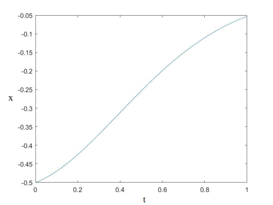
f=@(t,x) x^2*cos(x)-4*t*x; % differential equation
a=0; %interval
b=1;  
x0=-0.5; % initial condition
h=0.01; % step size
t=a:h:b; % generating time vector
n=length(t); % storing length of vector t
x=[x0 zeros(1,n-1)]; % initializing vector x
for i=1:n-1
k1=h*f(t(i),x(i)); % fourth order runge kutta equations
k2=h*f(t(i)+0.5*h,x(i)+0.5*k1);
k3=h*f(t(i)+0.5*h,x(i)+0.5*k2);
k4=h*f(t(i)+h,x(i)+k3);
k=(1/6)*(k1+2*k2+2*k3+k4);
x(i+1)=x(i)+k;
end
% plot(t,x) %plotting result
[t' x'] % displaying results

=====================

Output data format:

  [t x]

=============

0 -0.5000
0.0100 -0.4977
0.0200 -0.4952
0.0300 -0.4926
0.0400 -0.4898
0.0500 -0.4868
0.0600 -0.4837
0.0700 -0.4803
0.0800 -0.4769
0.0900 -0.4733
0.1000 -0.4695
0.1100 -0.4656
0.1200 -0.4615
0.1300 -0.4573
0.1400 -0.4530
0.1500 -0.4486
0.1600 -0.4440
0.1700 -0.4393
0.1800 -0.4345
0.1900 -0.4296
0.2000 -0.4246
0.2100 -0.4196
0.2200 -0.4144
0.2300 -0.4091
0.2400 -0.4038
0.2500 -0.3984
0.2600 -0.3929
0.2700 -0.3874
0.2800 -0.3818
0.2900 -0.3761
0.3000 -0.3704
0.3100 -0.3647
0.3200 -0.3589
0.3300 -0.3531
0.3400 -0.3472
0.3500 -0.3413
0.3600 -0.3355
0.3700 -0.3296
0.3800 -0.3237
0.3900 -0.3177
0.4000 -0.3118
0.4100 -0.3059
0.4200 -0.3000
0.4300 -0.2941
0.4400 -0.2882
0.4500 -0.2824
0.4600 -0.2765
0.4700 -0.2707
0.4800 -0.2649
0.4900 -0.2592
0.5000 -0.2535
0.5100 -0.2478
0.5200 -0.2422
0.5300 -0.2366
0.5400 -0.2311
0.5500 -0.2256
0.5600 -0.2202
0.5700 -0.2148
0.5800 -0.2095
0.5900 -0.2042
0.6000 -0.1990
0.6100 -0.1939
0.6200 -0.1888
0.6300 -0.1838
0.6400 -0.1789
0.6500 -0.1740
0.6600 -0.1692
0.6700 -0.1645
0.6800 -0.1599
0.6900 -0.1553
0.7000 -0.1508
0.7100 -0.1464
0.7200 -0.1421
0.7300 -0.1378
0.7400 -0.1337
0.7500 -0.1296
0.7600 -0.1256
0.7700 -0.1216
0.7800 -0.1178
0.7900 -0.1140
0.8000 -0.1103
0.8100 -0.1067
0.8200 -0.1032
0.8300 -0.0997
0.8400 -0.0963
0.8500 -0.0931
0.8600 -0.0898
0.8700 -0.0867
0.8800 -0.0837
0.8900 -0.0807
0.9000 -0.0778
0.9100 -0.0750
0.9200 -0.0722
0.9300 -0.0695
0.9400 -0.0669
0.9500 -0.0644
0.9600 -0.0620
0.9700 -0.0596
0.9800 -0.0573
0.9900 -0.0550
1.0000 -0.0529

Plot:

0.05 -0.1 -0.15 0.2 -0.25 0.3 0.35 0.4 0.45 0.5 0.2 0.4 0.6 0.8