Question

13 points) The horsepower (Y, in bhp) of a motor car engine was measured at a chosen set of values of running speed (X. In rpm). The data are given below (the first row is the running speed In rpm and the second row is the horsepower in bhp): rpm 1100 1700 2300 2700 3200 3500 4000 4800 5200 5600 6100 Horsepower (bhp) 44.32 77.51 102.98 122.76 151.11 158 202.8 220.29 266.28 286.63 297.03 The mean and sum of squares of the rpm are 3636.3636 rpm and 171940000.0000 rpm respectively, the mean of the horsepower values is 173.6100 bhp and the sum of the products of the two variables is 8299578.0000 rpm bhp. A scatterplot dis data is shown below: Car Engine Horsepower against Engine Running Speed 1000 2000 3000 4000 5000 1000 Engine running speed from Please provide answers to the following to 3 decimals places where appropriate

Part a)

Compute the regression line for these data, and provide your estimates of the slope and intercept parameters. Please round intermediate results to 6 decimal places.

Slope:

Intercept:

Note: For sub-parts below, use the slope and intercept values in Part a, corrected to 3 decimal places to calculate answers by hand using a scientific calculator.

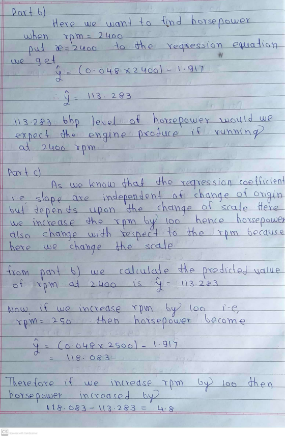
Part b)

Based on the regression model, what level of horsepower would you expect the engine to produce if running at 24002400 rpm?

Answer:

Part c)

Assuming the model you have fitted, if increase the running speed by 100100 rpm, what would you expect the change in horsepower to be?

Answer:

Part d)

The standard error of the estimate of the slope coefficient was found to be 0.0013570.001357. Provide a 95% confidence interval for the true underlying slope.

Confidence interval: (  ,  )

Part e)

Without extending beyond the existing range of speed values or changing the number of observations, we would expect that increasing the variance of the rpm speeds at which the horsepower levels were found would make the confidence interval in (d)

A. either wider or narrower depending on the values chosen.
B. narrower.
C. unchanged.
D. wider.


Part f)

If testing the null hypothesis that horsepower does not depend linearly on rpm, what would be your test statistic? (For this part, you are to calculate the test statistic by hand using appropriate values from the answers you provided in part (a) accurate to 3 decimal places, and values given to you in part (d).)

Answer:

Part g)

Assuming the test is at the 1% significance level, what would you conclude from the above hypothesis test?

A. Since the observed test statistic falls in either the upper or lower 1/2 percentiles of the t distribution with 99 degrees of freedom, we can reject the null hypothesis that the horsepower does not depend linearly on rpm.
B. Since the observed test statistic does not fall in either the upper or lower 1/2 percentiles of the t distribution with 99 degrees of freedom, we cannot reject the null hypothesis that the horsepower does not depend linearly on rpm.
C. Since the observed test statistic does not fall in either the upper or lower 1 percentiles of the t distribution with 99 degrees of freedom, we cannot reject the null hypothesis that the horsepower does not depend linearly on rpm.
D. Since the observed test statistic does not fall in either the upper or lower 1/2 percentiles of the t distribution with 99 degrees of freedom, we can reject the null hypothesis that the horsepower does not depend linearly on rpm.
E. Since the observed test statistic falls in either the upper or lower 1/2 percentiles of the t distribution with 99 degrees of freedom, we cannot reject the null hypothesis that the horsepower does not depend linearly on rpm.

Answer 1

we have given that 2 de = 36 36 3636 rpm ECHi-æ)2 = 171940000. 0000 rpm 7 = 173. 61ool E Capi-D) (Li-I) = 8299578. 0000 rpm Ohp h = 11 regress- 6 de are part a) Now we know that ý = a + bae be the estimated regression equation of line of ion y on where a and obtained by the method of least squares enor sum of square then and b= 6 = Ecæi-e) (Li-y) (xi-2012 with minimizing a=j-ba b= 82 99578.0000 1719 40 000 0000 6=0.048270 а: у- bx = (173.6100)- (0.04.8270 x 36 36.3636) = -1.917271 .. Equation of line of regression you de ĝ = (0.048270) + - 1.917271 slope=6= 0.048270 - intercepta a = -1.917271 CS Scanned with CamScanner

Part 6) Here we want to find horsepower when rpm = 2400 put x= 2400 to the regression equation we get | 1 (0 0 4 8 2 40o) - -917 ĝ 113. 283 113.283 the level of horsepower would we expect the engine produce if oning runn at 2400 rpm. the 100 rpm by rpm because part c) As we know that the regression coefficient le slope are independent of change of origin but depends upon the change of scale Here we increase hence horsepower also change with respect to the here we change the scale. from part 6) we calculate the predicted value is ý = Now if we increase rpm by 100 |-е, then horsepower become ŷ - (0.048x25001 - 1.917 of rpm at 2400 = 113.203 rpm = 250 118. 083 horsepower Therefore if we increase rpm by 100 then increased by 118.083 - 113.283 = CS Scanned with CamScanner

horsepower will be increased by 4.8 bhp part d) know loo(1-2% confidence interval for slope is given as (6. tn 2,42 se (6) 6+ tn-2d/2 se (6) have bi 0.048 se(6) 0.001357 Here we have to find 95% confidence interval for slope tn-2 2/2 = t 11-20 tg.o.os tgo.025 = 2.262 2 2 6- tn 2,42 se(6) - lower bound for (- 0.048 - (2 2-262 x 0. 001357) 0.045 Upper bound 6+ tn 2,412 se (6) for C. (2.262 X0.001357) = 0.048 = 0.0 51 95% confidence interval for slope is 0.045 0.051) given as CS Scanned with CamScanner

t table as follows:

7:43 62.0 KB/S 774 Edit 26 Х t-distribution Confidence Level 85% 90% 95% 98% 60% 70% 80% 99% 99.8% 99.9% 2 Tailed 1 Tailed 0.40 0.20 0.30 0.15 0.20 0.10 Level of Significance 0.15 0.10 0.05 0.02 0.075 0.05 0.025 0.01 0.01 0.005 0.002 0.001 0.001 0.0005 26.30 12.39 8.499 6.835 5.946 5.403 5.039 0.039 4.780 2.822 3.250 df 1 2 3 4 5 6 7 8 9 10 11 12 13 13 14 15 16 17 18 19 20 21 22 23 24 25 4.586 4.437 1.376 1.963 3.133 4.195 6.320 12.69 31.81 63.67 1.060 1.385 1.883 2.278 2.912 4.271 4.271 6.816 9.520 0.978 1.250 1.637 1.924 2.352 3.179 4.525 5.797 0.941 1.190 1.533 1.778 2.132 2.776 3.744 4.596 0.919 1.156 1.476 1.699 2.015 2.570 3.365 4.030 0.906 1.134 1.440 1.650 1.943 2.447 3.143 3.707 0.896 1.119 1.415 1.617 1.895 2.365 2.999 3.500 0.889 1.108 0.00% 1.397 1.592 1.860 2.306 2.897 3.356 0.000 0.883 1.100 1.383 1.574 1.833 2.262 0.879 1.372 1.093 V. 1.559 1.813 2.228 2.764 3.170 0.875 0.00 1.088 1.363 1.305 1.548 1.796 2.201 2.719 3.106 0.873 1.083 1.356 1.538 1.782 2.179 2.682 3.055 0.870 1.079 1.350 1.530 1.771 2.160 2.651 3.013 0 000 0.868 1.076 1.345 1.523 1.761 . 15 2.145 2.625 2.977 0.866 1.074 1.341 1.517 1.753 2.131 2.603 2.947 0.865 1.071 1.337 1.512 1.746 2.120 2.584 2.921 0.863 1.069 1.333 1.508 1.740 2.110 2.567 2.899 0.862 1.067 1.330 1.504 1.734 2.101 2.553 2.879 0.861 1.000 1.066 1.328 1.500 1.000 1.729 2.095 2.093 2.540 2.861 0.860 1.064 1.325 1.497 19 1.725 .125 2.086 2.529 2.840 0.859 1.063 1.323 1.494 1.721 2.080 2.518 2.832 0.858 1.061 1.321 1.717 2.074 2.074 2.509 2.819 0.857 1.060 1.319 1.489 1.714 2.069 2.500 2.808 0.857 1.487 1.711 2.064 2.493 2.797 0.856 1.058 1.485 1.708 2.060 2.486 2.788 0.856 1.058 1.315 1492 1.483 1.706 2.056 2.479 2.779 0.855 1.057 1.314 ora 1.482 1.703 2.052 2.473 more 2.473 2.771 1994 0.855 1.056 1.313 1.480 1.701 2.048 2.468 2.764 MORALES 1120 1.055 Icon 0.854 1.311 1.479 1.699 2.045 2.463 2.757 LE 0.854 1.055 1.310 2019 20 1.477 1.697 Movie 2.042 2.458 2.750 0.851 1.050 1.303 Tied 10 201 202 203 1.468 1.684 2.021 2.424 2.705 dou 0 0 100 0.849 1.047 1.299 1.462 1.676 2.009 2.404 2.678 0.848 0 1 1.045 1.296 1.458 1.671 2.000 2.391 2.661 0.847 1.044 1.294 1.456 1.667 1.994 2.381 2.648 0.846 1.043 1.292 1.453 1.664 1.990 2.374 2.639 0.846 1.042 1.291 1.452 1.662 1.987 2.369 2.632 0.845 1.042 1.290 1.451 1.660 1.984 2.365 2.626 19.65 9.937 7.115 5.876 5.201 4.783 4.500 4.297 4.297 4.144 4.025 3.930 3.930 3.852 3.788 3.733 3.687 3.646 3.611 3.580 4.318 4.221 4.141 4.073 4.015 3.965 3.922 3.884 3.850 3.552 3.820 1.492 1.059 1.318 1.316 27 28 29 30 40 50 60 70 80 90 100 3.528 3.505 3.485 3.467 3.451 3.435 3.421 3.409 3.397 3.386 3.307 3.262 3.232 3.211 3.196 3.184 3.174 3.792 3.768 3.746 3.725 2707 3.707 con 3.690 3.674 3.660 3.646 3.551 3.496 3.460 10 3.435 3.417 3.402 3.391 0842 1.036 1.282 1.440 1.645 1.960 2.327 2.576 3.091 3.291 סס w DD Tools Mobile View Share PDF to DOC