Question

methodology of fourier series questions and solution in matlap and show result and discussion.

Choose any question you like.

Answer 1

About Fourier Series Models

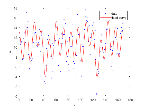
The Fourier series is a sum of sine and cosine functions that describes a periodic signal. It is represented in either the trigonometric form or the exponential form. The toolbox provides this trigonometric Fourier series form

y=a0+ni=1aicos(iwx)+bisin(iwx)

where a0 models a constant (intercept) term in the data and is associated with the i = 0 cosine term, wis the fundamental frequency of the signal, n is the number of terms (harmonics) in the series, and 1 ≤ n ≤ 8.

For more information about the Fourier series, refer to Fourier Analysis and Filtering (MATLAB).

Fit Fourier Models Interactively

1. Open the Curve Fitting app by entering cftool. Alternatively, click Curve Fitting on the Apps tab.

2. In the Curve Fitting app, select curve data (X data and Y data, or just Y data against index).

   Curve Fitting app creates the default curve fit, Polynomial.

3. Change the model type from Polynomial to Fourier.

Fourier Number of terms: 1 Equation: a0 + al*cos(x*w) + bl*sin(x*w) Center and scale Fit Options...

You can specify the following options:

• Choose the number of terms: 1 to 8.

  Look in the Results pane to see the model terms, the values of the coefficients, and the goodness-of-fit statistics.

• (Optional) Click Fit Options to specify coefficient starting values and constraint bounds, or change algorithm settings.

  The toolbox calculates optimized start points for Fourier series models, based on the current data set. You can override the start points and specify your own values in the Fit Options dialog box.

  For more information on the settings, see Specifying Fit Options and Optimized Starting Points.

For an example comparing the library Fourier fit with custom equations, see Custom Nonlinear ENSO Data Analysis.

Fit Fourier Models Using the fit Function

View MATLAB Command

This example shows how to use the fit function to fit a Fourier model to data.

The Fourier library model is an input argument to the fit and fittype functions. Specify the model type fourier followed by the number of terms, e.g., 'fourier1' to 'fourier8' .

This example fits the El Nino-Southern Oscillation (ENSO) data. The ENSO data consists of monthly averaged atmospheric pressure differences between Easter Island and Darwin, Australia. This difference drives the trade winds in the southern hemisphere.

The ENSO data is clearly periodic, which suggests it can be described by a Fourier series. Use Fourier series models to look for periodicity.

Fit a Two-Term Fourier Model

Load some data and fit an two-term Fourier model.

load enso;
f = fit(month,pressure,'fourier2')

f = 
     General model Fourier2:
     f(x) =  a0 + a1*cos(x*w) + b1*sin(x*w) + 
               a2*cos(2*x*w) + b2*sin(2*x*w)
     Coefficients (with 95% confidence bounds):
       a0 =       10.63  (10.23, 11.03)
       a1 =       2.923  (2.27, 3.576)
       b1 =       1.059  (0.01593, 2.101)
       a2 =     -0.5052  (-1.086, 0.07532)
       b2 =      0.2187  (-0.4202, 0.8576)
       w =      0.5258  (0.5222, 0.5294)

plot(f,month,pressure)

8 data fitted curve 16 14 N 10 y 8 6 4 2 0 0 20 40 60 80 100 120 140 160 180 X

The confidence bounds on a2 and b2 cross zero. For linear terms, you cannot be sure that these coefficients differ from zero, so they are not helping with the fit. This means that this two term model is probably no better than a one term model.

Measure Period

The w term is a measure of period. 2*pi/wconverts to the period in months, because the period of sin() and cos() is 2*pi .

w = f.w

w = 0.5258

2*pi/w

ans = 11.9497

w is very close to 12 months, indicating a yearly period. Observe this looks correct on the plot, with peaks approximately 12 months apart.

Fit an Eight-Term Fourier Model

f2 = fit(month,pressure,'fourier8')

f2 = 
     General model Fourier8:
     f2(x) = 
               a0 + a1*cos(x*w) + b1*sin(x*w) + 
               a2*cos(2*x*w) + b2*sin(2*x*w) + a3*cos(3*x*w) + b3*sin(3*x*w) + 
               a4*cos(4*x*w) + b4*sin(4*x*w) + a5*cos(5*x*w) + b5*sin(5*x*w) + 
               a6*cos(6*x*w) + b6*sin(6*x*w) + a7*cos(7*x*w) + b7*sin(7*x*w) + 
               a8*cos(8*x*w) + b8*sin(8*x*w)
     Coefficients (with 95% confidence bounds):
       a0 =       10.63  (10.28, 10.97)
       a1 =      0.5668  (0.07981, 1.054)
       b1 =      0.1969  (-0.2929, 0.6867)
       a2 =      -1.203  (-1.69, -0.7161)
       b2 =     -0.8087  (-1.311, -0.3065)
       a3 =      0.9321  (0.4277, 1.436)
       b3 =      0.7602  (0.2587, 1.262)
       a4 =     -0.6653  (-1.152, -0.1788)
       b4 =     -0.2038  (-0.703, 0.2954)
       a5 =    -0.02919  (-0.5158, 0.4575)
       b5 =     -0.3701  (-0.8594, 0.1192)
       a6 =    -0.04856  (-0.5482, 0.4511)
       b6 =     -0.1368  (-0.6317, 0.3581)
       a7 =       2.811  (2.174, 3.449)
       b7 =       1.334  (0.3686, 2.3)
       a8 =     0.07979  (-0.4329, 0.5925)
       b8 =     -0.1076  (-0.6037, 0.3885)
       w =     0.07527  (0.07476, 0.07578)

plot(f2,month,pressure)

8 data fitted curve 16 14 N 10 y 8 6 4 2 0 0 20 40 60 80 100 120 140 160 180 X

Measure Period

w = f2.w

w = 0.0753

(2*pi)/w

ans = 83.4736

With the f2 model, the period w is approximately 7 years.

Examine Terms

Look for the coefficients with the largest magnitude to find the most important terms.

• a7 and b7 are the largest. Look at the a7 term in the model equation: a7*cos(7*x*w). 7*w== 7/7 = 1 year cycle. a7 and b7 indicate the annual cycle is the strongest.

• Similarly, a1 and b1 terms give 7/1, indicating a seven year cycle.

• a2 and b2 terms are a 3.5 year cycle (7/2). This is stronger than the 7 year cycle because the a2and b2 coefficients have larger magnitude than a1 and b1.

• a3 and b3 are quite strong terms indicating a 7/3 or 2.3 year cycle.

• Smaller terms are less important for the fit, such as a6, b6, a5, and b5.

Typically, the El Nino warming happens at irregular intervals of two to seven years, and lasts nine months to two years. The average period length is five years. The model results reflect some of these periods.

Set Start Points

The toolbox calculates optimized start points for Fourier fits, based on the current data set. Fourier series models are particularly sensitive to starting points, and the optimized values might be accurate for only a few terms in the associated equations. You can override the start points and specify your own values.

After examining the terms and plots, it looks like a 4 year cycle might be present. Try to confirm this by setting w. Get a value for w, where 8 years = 96 months.

w = (2*pi)/96

w = 0.0654

Find the order of the entries for coefficients in the model ('f2') by using the coeffnames function.

coeffnames(f2)

ans = 18x1 cell
    {'a0'}
    {'a1'}
    {'b1'}
    {'a2'}
    {'b2'}
    {'a3'}
    {'b3'}
    {'a4'}
    {'b4'}
    {'a5'}
    {'b5'}
    {'a6'}
    {'b6'}
    {'a7'}
    {'b7'}
    {'a8'}
    {'b8'}
    {'w' }

Get the current coefficient values.

coeffs = coeffvalues(f2)

coeffs = 1×18

   10.6261    0.5668    0.1969   -1.2031   -0.8087    0.9321    0.7602   -0.6653   -0.2038   -0.0292   -0.3701   -0.0486   -0.1368    2.8112    1.3344    0.0798   -0.1076    0.0753

Set the last coefficient, w, to 0.065.

coeffs(:,18) = w

coeffs = 1×18

   10.6261    0.5668    0.1969   -1.2031   -0.8087    0.9321    0.7602   -0.6653   -0.2038   -0.0292   -0.3701   -0.0486   -0.1368    2.8112    1.3344    0.0798   -0.1076    0.0654

Set the start points for coefficients using the new value for w.

f3 = fit(month,pressure,'fourier8', 'StartPoint', coeffs);

Plot both fits to see that the new value for w in f3does not produce a better fit than f2 .

plot(f3,month,pressure)
hold on
plot(f2, 'b')
hold off
legend( 'Data', 'f3', 'f2')

8 16 Data - 13 12 14 N 10 y 8 6 4 2 0 0 20 40 60 80 100 120 140 160 180 X

Find Fourier Fit Options

Find available fit options using fitoptions(modelname), where modelname is the model type fourier followed by the number of terms, e.g., 'fourier1' to 'fourier8' .

fitoptions('fourier8')

ans =

        Normalize: 'off'
          Exclude: []
          Weights: []
           Method: 'NonlinearLeastSquares'
           Robust: 'Off'
       StartPoint: [1x0 double]
            Lower: [1x0 double]
            Upper: [1x0 double]
        Algorithm: 'Trust-Region'
    DiffMinChange: 1.0000e-08
    DiffMaxChange: 0.1000
          Display: 'Notify'
      MaxFunEvals: 600
          MaxIter: 400
           TolFun: 1.0000e-06
             TolX: 1.0000e-06

If you want to modify fit options such as coefficient starting values and constraint bounds appropriate for your data, or change algorithm settings, see the options for NonlinearLeastSquares on the fitoptions reference page.