Question

Hello

These are a math problems that need to solve by MATLAB as code

Thank you !

Initial Value Problem #1: Consider the following first order ODE: dy-p-3 from to 2.2 with y() I (a) Solve with Euler's explicit method using h04. (b) Solve with the midpoint method using h 0.4. (c) Solve with the classical fourth-order Runge-Kutta method using 0.4 analytical solution of the ODE is,·? solution and the numerical solution at the points where the numerical solution is determined +In each part, calculate the error between the true Initial Value Problem #2: Consider the differential equation for mass-spring-damper system as shown: where k2 - 48 N/m/kg, y07s, x(0)0, and d0.2 m/s. Solve the ODE over the interva dt dx 031s5 s, and pla (two separate figures on one page) as a function of t. 1.) Write the second order ODE as a system of first order ODEs 2.) Solve for step size t = 0.1 seconds 3.) Provide brief discussion of the physics (derivation of governing equation) and explanation of the results

Answer 1

Note: More than one question asked. So I did first part.

Copyable Code:

Part (a):

function.m

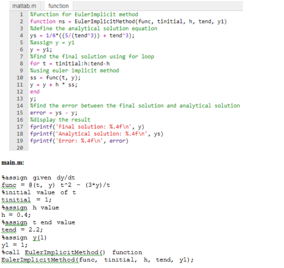
%function for EulerImplicit method
function ns = EulerImplicitMethod(func, tinitial, h, tend, y1)
%define the analytical solution equation
ys = 1/6*((5/(tend^3)) + tend^3);
%assign y = y1
y = y1;
%find the final solution using for loop
for t = tinitial:h:tend-h
%using euler implicit method
ss = func(t, y);
y = y + h * ss;
end
y;
%find the error between the final solution and analytical solution
error = ys - y;
%display the result
fprintf('Final solution: %.4f\n', y)
fprintf('Analytical solution: %.4f\n', ys)
fprintf('Error: %.4f\n', error)

main.m:

%assign given dy/dt
func = @(t, y) t^2 - (3*y)/t
%initial value of t
tinitial = 1;
%assign h value
h = 0.4;
%assign t end value
tend = 2.2;
%assign y(1)
y1 = 1;
%call EulerImplicitMethod() function
EulerImplicitMethod(func, tinitial, h, tend, y1);

Part (b)

function.m

%function for MidPointMethod method
function ns = MidPointMethod(func, tinitial, h, tend, y1)
%define the analytical solution equation
ys = 1/6*((5/(tend^3)) + tend^3);
%assign y = y1
y = y1;
%find the final solution using for loop
for t = tinitial:h:tend-h
%using midpoint method
ss = func(t, y);
ss1 = func(t+h/2, y+h*ss/2);
y = y + h * ss1;
end
y;
%find the error between the final solution and analytical solution
error = ys - y;
%display the result
fprintf('Final solution: %.4f\n', y)
fprintf('Analytical solution: %.4f\n', ys)
fprintf('Error: %.4f\n', error)

main.m:

%assign given dy/dt

func = @(t, y) t^2 - (3*y)/t
%initial value of t
tinitial = 1;
%assign h value
h = 0.4;
%assign t end value
tend = 2.2;
%assign y(1)
y1 = 1;
%call MidPointMethod() function
MidPointMethod(func, tinitial, h, tend, y1);

Part (c)

function.m

%function for RungeKuttaMethod
function ns = RungeKuttaMethod(func, tinitial, h, tend, y1)
%define the analytical solution equation
ys = 1/6*((5/(tend^3)) + tend^3);
%assign y = y1
y = y1;
%find the final solution using for loop
for t = tinitial:h:tend-h
%using runge kutta method
ss = func(t, y);
ss1 = func(t+h/2, y+h*ss/2);
ss2 = func(t+h/2, y+h*ss1/2);
ss3 = func(t+h, y+h*ss2);
y = y + h * (ss + 2*ss1 + 2*ss2 + ss3)/6;
end
y;
%find the error between the final solution and analytical solution
error = ys - y;
%display the result
fprintf('Final solution: %.4f\n', y)
fprintf('Analytical solution: %.4f\n', ys)
fprintf('Error: %.4f\n', error)

main.m:

%assign given dy/dt
func = @(t, y) t^2 - (3*y)/t
%initial value of t
tinitial = 1;
%assign h value
h = 0.4;
%assign t end value
tend = 2.2;
%assign y(1)
y1 = 1;
%call RungeKuttaMethod() function
RungeKuttaMethod(func, tinitial, h, tend, y1);