
Homework Answers
![%&Matlab function for bisection method function [root,count] bisection method (fun, a,b) %f(al) should be positive f (b1) sho](http://img.homeworklib.com/questions/3312ac50-a4a2-11eb-9cbb-014212f7f953.png?x-oss-process=image/resize,w_560)
![else hold off end axis ([tval(1)-dt/2,tval(end)+dt/2,yval(1)-dy/2, yval(end) +dy/2]) end 888888888888888 End of Code 88888868](http://img.homeworklib.com/questions/339e5170-a4a2-11eb-bbc9-ff37817e309f.png?x-oss-process=image/resize,w_560)
%%Matlab code for Direction field and solution of ODE
clear all
close all
%function of 1st order diffrential eqn
f = @(g) 1-g+((0.2*g.^2)./(1+0.01.*g.^2));
%plotting of R.H.S of the function
gg=-5:0.1:20;
f_gg=f(gg);
plot(gg,f_gg)
grid on
title('plotting of R.H.S of the function')
xlabel('g')
ylabel('f(g)')
%Finding the location for which function f crosses zero
%Here we will going to use Bisection method to find the root
%all initial guess
a=[0 7 7];
b=[3 3 20];
fprintf('For the function \n')
disp(f)
fprintf('The roots are \n')
fprintf('\ta\tb\troot\n')
for i=1:length(a)
[root1,count1]=bisection_method(f,a(i),b(i));
fprintf('\t%0.2f\t%0.2f\t%f\t\n',a(i),b(i),root1)
end
fprintf('Here a and b are intervals\n')
%function of 1st order diffrential eqn
fun = @(t,g) 1-g+((0.2*g.^2)./(1+0.01.*g.^2));
%solution of differential equation using Runge Kutta 4
%step size
h=0.01;
%all final t steps
t1=0;tn=20;
t_in=t1; %Initial
t
t_max=tn; %Final t
%Runge Kutta 4 iterations
n=(t_max-t_in)/h;
g_rk(1)=10; %initial g
t_rk(1)=t1;
%RK4 iterations
for i=1:n
k0=h*fun(t_rk(i),g_rk(i));
k1=h*fun(t_rk(i)+(1/2)*h,g_rk(i)+(1/2)*k0);
k2=h*fun(t_rk(i)+(1/2)*h,g_rk(i)+(1/2)*k1);
k3=h*fun(t_rk(i)+h,g_rk(i)+k2);
t_rk(i+1)=t_in+i*h;
g_rk(i+1)=double(g_rk(i)+(1/6)*(k0+2*k1+2*k2+k3));
end
figure(2)
plot(t_rk,g_rk)
ylabel('g(t)')
xlabel('t')
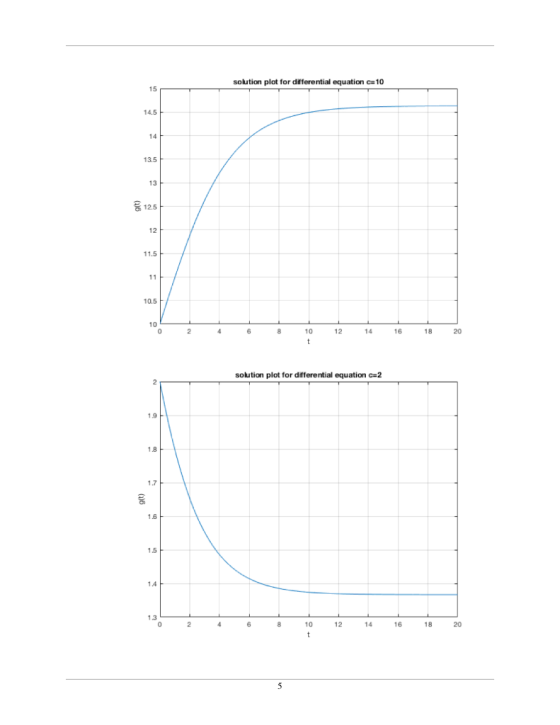
title('solution plot for differential equation c=10')
grid on
clear t_rk; clear g_rk
%solution of differential equation using Runge Kutta 4
%step size
h=0.01;
%all final t steps
t1=0;tn=20;
t_in=t1; %Initial
t
t_max=tn; %Final t
%Runge Kutta 4 iterations
n=(t_max-t_in)/h;
g_rk(1)=2; %initial g
t_rk(1)=t1;
%RK4 iterations
for i=1:n
k0=h*fun(t_rk(i),g_rk(i));
k1=h*fun(t_rk(i)+(1/2)*h,g_rk(i)+(1/2)*k0);
k2=h*fun(t_rk(i)+(1/2)*h,g_rk(i)+(1/2)*k1);
k3=h*fun(t_rk(i)+h,g_rk(i)+k2);
t_rk(i+1)=t_in+i*h;
g_rk(i+1)=double(g_rk(i)+(1/6)*(k0+2*k1+2*k2+k3));
end
figure(3)
plot(t_rk,g_rk)
ylabel('g(t)')
xlabel('t')
title('solution plot for differential equation c=2')
grid on
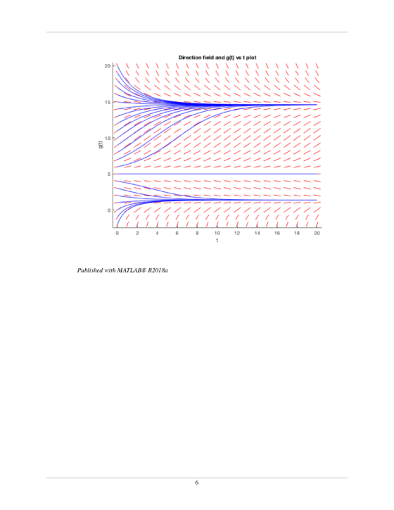
%code for direction field
figure(4)
hold on
%plotting dir field for differential equation
dirfield(fun,0:1:20,-2:1:20)
%Findind solution for all initial condition -2:2
for y0=-2:1:20
%solution using matlab inbuilt ode45 function
[xs,ys] = ode45(fun,[0,20],y0);
%plotting of solution
plot(xs,ys,'b')
end
hold off
xlabel('t')
ylabel('g(t)')
title('Direction field and g(t) vs t plot')
%%Matlab function for bisection method
function [root,count]=bisection_method(fun,a,b)
%f(a1) should be positive
%f(b1) should be negative
count=0;
k=10;
%loop for bisection method
while k>10^-6
count=count+1;
xx(count)=(a+b)/2;
mm=double(fun(xx(count)));
if mm>=0
a=xx(count);
else
b=xx(count);
end
k=abs(a-b);
end
root=xx(end);
end
%function for plotting direction field
function dirfield(f,tval,yval)
% dirfield(f, t1:dt:t2, y1:dy:y2)
%
% plot direction field for first order ODE y' =
f(t,y)
% using t-values from t1 to t2 with spacing of dt
% using y-values from y1 to t2 with spacing of dy
%
% f is an @ function, or an inline function,
% or the name of an m-file with
quotes.
%
% Example: y' = -y^2 + t
% Show direction field for t in [-1,3], y in [-2,2],
use
% spacing of .2 for both t and y:
%
% f = @(t,y) -y^2+t
% dirfield(f, -1:.2:3, -2:.2:2)
[tm,ym]=meshgrid(tval,yval);
dt = tval(2) - tval(1);
dy = yval(2) - yval(1);
fv = vectorize(f);
if isa(f,'function_handle')
fv = eval(fv);
end
yp=feval(fv,tm,ym);
s = 1./max(1/dt,abs(yp)./dy)*0.35;
h = ishold;
quiver(tval,yval,s,s.*yp,0,'.r'); hold on;
quiver(tval,yval,-s,-s.*yp,0,'.r');
if h
hold on
else
hold off
end
axis([tval(1)-dt/2,tval(end)+dt/2,yval(1)-dy/2,yval(end)+dy/2])
end
%%%%%%%%%%%%%%%%%%% End of Code %%%%%%%%%%%%%%%%
Add Answer to:
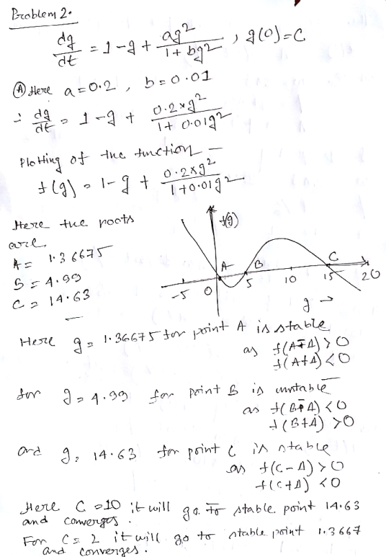
Problem 2: consider the non-dimensionalized model for dynamic protein concentration: 2.g(0)-c A) Use qualitative analysis (plot...
2. Consider the basic Solow model in our textbook. (a) As before suppose f(0) 0, but...
 2. Consider the basic Solow model in our textbook. (a) As before suppose f(0) 0, but suppose that one of the Inada conditions do not hold. In particular, suppose limk--0/(k) → c where c > 0 is a constant. (Recall f"(k) is the derivative of the intensive production function and is equal to the marginal product of capital.) Describe all the cases using diagrams (which has savings and the investment breakeven lines) to explain the paths of the economy starting...
2. Points = 26. Consider Market Model: Demand: Supply: Q=a-bP Q=-c+dP (a, b>0) (c,d > 0) 1) Discuss in words the...
 2. Points = 26. Consider Market Model: Demand: Supply: Q=a-bP Q=-c+dP (a, b>0) (c,d > 0) 1) Discuss in words the meaning of each equation in the model (3 points); 2) Find the equilibrium levels of P* and Q* (3 points); 3) Draw qualitative conclusions about changes in P* and Q* when each of the parameters change. (Qualitative conclusion shows the direction of change.) Explain economic meaning of these changes. (Total 6 points: 3 points for P*; 3 points for...
2. Consider Market Model (а, b > 0) (c, d >0) Demand: Q%3Dа — БР Q%3D-с...
 2. Consider Market Model (а, b > 0) (c, d >0) Demand: Q%3Dа — БР Q%3D-с + dP Supply: 1) Discuss in words the meaning of each equation in the model 2) Find the equilibrium levels of P and Q* 3) Draw gualitative conclusions about changes in P* and Q' when each of the parameters change. (Qualitative conclusion shows the direction of change.) Explain economic meaning of these changes 4) If a 10, c 5, b = 2; d =...
Just 5-8 1 Analytics of the Solow Model In the Solow economy, people consume a good...
 Just 5-8
1 Analytics of the Solow Model In the Solow economy, people consume a good that firms produce with technology Y (which we assume to be constant) and f is a Cobb-Douglas production function Af (K, L), where A is TFP f(K, L) KL-a Here K is the stock of capital, which depreciates at rate δ E (0, 1) per period, and L is the labor force, which grows exogenously at rate n > 0. Here employment is always...
Just 5-8
1 Analytics of the Solow Model In the Solow economy, people consume a good that firms produce with technology Y (which we assume to be constant) and f is a Cobb-Douglas production function Af (K, L), where A is TFP f(K, L) KL-a Here K is the stock of capital, which depreciates at rate δ E (0, 1) per period, and L is the labor force, which grows exogenously at rate n > 0. Here employment is always...
please, i need answeer for all 4 questions Consider National-Income Model: National Income: Consumption: Investment: Government...
 please, i need answeer for all 4 questions
Consider National-Income Model: National Income: Consumption: Investment: Government Sector: Taxes: Y=C+I+G C = a + b (Y-T) I=k+rY G=Go T=f+jY 0<b<1 0<x<1 a> 0 in mln dollars; k>0 in mln dollars; Go > in mln dollars f> 0 in mln dollars; 0<j<1 1) Discuss in words the meaning of each of the equations in the model (3 points); 2) Find the equilibrium level of GDP (Y) in reduced form (3 points); 3)...
please, i need answeer for all 4 questions
Consider National-Income Model: National Income: Consumption: Investment: Government Sector: Taxes: Y=C+I+G C = a + b (Y-T) I=k+rY G=Go T=f+jY 0<b<1 0<x<1 a> 0 in mln dollars; k>0 in mln dollars; Go > in mln dollars f> 0 in mln dollars; 0<j<1 1) Discuss in words the meaning of each of the equations in the model (3 points); 2) Find the equilibrium level of GDP (Y) in reduced form (3 points); 3)...
6. Consider the Cauchy problem for the advection equation, u +cu0, where c>0 a) Expand u(z,t + k) in a Taylor series up to O(k3) terms. Then use the advection equation to obtain c2k2 uzz(x, t)...
 6. Consider the Cauchy problem for the advection equation, u +cu0, where c>0 a) Expand u(z,t + k) in a Taylor series up to O(k3) terms. Then use the advection equation to obtain c2k2 uzz(x, t) + O(k"). u(z, t + k) u(x, t) _ cku(x, t) +- b) Replace u and ur by centered difference approximations to obtain the explicit scheme This is the Lax-Wendroff method. It is von Neumann stable for 0 < 8 < 1 and it...
USU.US CUJL 1.ULTIUZULUV.CUIT 1. Points = 18 Consider National-Income Model: National Income: Consumption: Investment: Government Sector:...
 USU.US CUJL 1.ULTIUZULUV.CUIT 1. Points = 18 Consider National-Income Model: National Income: Consumption: Investment: Government Sector: Taxes: Y=C+I+G C = a + b (Y-T) I=k+rY G=Go T=f+jY 0<b<1 0<r<1 a> 0 in mln dollars; k>0 in mln dollars; Go >O in mln dollars f> 0 in mln dollars; 0<j<1 1) Discuss in words the meaning of each of the equations in the model (3 points); 2) Find the equilibrium level of GDP (Y) in reduced form (3 points); 3) If...
in matlab -Consider the equation f(x) = x-2-sin x = 0 on the interval x E [0.1,4 π] Use a plot to approximately locate the roots of f. To which roots do the fol- owing initial guesses converge wh...
 in
matlab
-Consider the equation f(x) = x-2-sin x = 0 on the interval x E [0.1,4 π] Use a plot to approximately locate the roots of f. To which roots do the fol- owing initial guesses converge when using Function 4.3.1? Is the root obtained the one that is closest to that guess? )xo = 1.5, (b) x0 = 2, (c) x.-3.2, (d) xo = 4, (e) xo = 5, (f) xo = 27. Function 4.3.1 (newton) Newton's method...
in
matlab
-Consider the equation f(x) = x-2-sin x = 0 on the interval x E [0.1,4 π] Use a plot to approximately locate the roots of f. To which roots do the fol- owing initial guesses converge when using Function 4.3.1? Is the root obtained the one that is closest to that guess? )xo = 1.5, (b) x0 = 2, (c) x.-3.2, (d) xo = 4, (e) xo = 5, (f) xo = 27. Function 4.3.1 (newton) Newton's method...
Based on the document below, 1. Describe the hypothesis Chaudhuri et al ids attempting to evaluate;...
 Based on the document below,
1. Describe the hypothesis Chaudhuri et al ids attempting to
evaluate; in other words, what is the goal of this paper? Why is he
writing it?
2. Does the data presented in the paper support the hypothesis
stated in the introduction? Explain.
3.According to Chaudhuri, what is the potential role of thew
alkaline phosphatase in the cleanup of industrial waste.
CHAUDHURI et al: KINETIC BEHAVIOUR OF CALF INTESTINAL ALP WITH PNPP 8.5, 9, 9.5, 10,...
Based on the document below,
1. Describe the hypothesis Chaudhuri et al ids attempting to
evaluate; in other words, what is the goal of this paper? Why is he
writing it?
2. Does the data presented in the paper support the hypothesis
stated in the introduction? Explain.
3.According to Chaudhuri, what is the potential role of thew
alkaline phosphatase in the cleanup of industrial waste.
CHAUDHURI et al: KINETIC BEHAVIOUR OF CALF INTESTINAL ALP WITH PNPP 8.5, 9, 9.5, 10,...
 2. Consider the basic Solow model in our textbook. (a) As before suppose f(0) 0, but suppose that one of the Inada conditions do not hold. In particular, suppose limk--0/(k) → c where c > 0 is a constant. (Recall f"(k) is the derivative of the intensive production function and is equal to the marginal product of capital.) Describe all the cases using diagrams (which has savings and the investment breakeven lines) to explain the paths of the economy starting...
 2. Points = 26. Consider Market Model: Demand: Supply: Q=a-bP Q=-c+dP (a, b>0) (c,d > 0) 1) Discuss in words the meaning of each equation in the model (3 points); 2) Find the equilibrium levels of P* and Q* (3 points); 3) Draw qualitative conclusions about changes in P* and Q* when each of the parameters change. (Qualitative conclusion shows the direction of change.) Explain economic meaning of these changes. (Total 6 points: 3 points for P*; 3 points for...
 2. Consider Market Model (а, b > 0) (c, d >0) Demand: Q%3Dа — БР Q%3D-с + dP Supply: 1) Discuss in words the meaning of each equation in the model 2) Find the equilibrium levels of P and Q* 3) Draw gualitative conclusions about changes in P* and Q' when each of the parameters change. (Qualitative conclusion shows the direction of change.) Explain economic meaning of these changes 4) If a 10, c 5, b = 2; d =...
 Just 5-8
1 Analytics of the Solow Model In the Solow economy, people consume a good that firms produce with technology Y (which we assume to be constant) and f is a Cobb-Douglas production function Af (K, L), where A is TFP f(K, L) KL-a Here K is the stock of capital, which depreciates at rate δ E (0, 1) per period, and L is the labor force, which grows exogenously at rate n > 0. Here employment is always...
Just 5-8
1 Analytics of the Solow Model In the Solow economy, people consume a good that firms produce with technology Y (which we assume to be constant) and f is a Cobb-Douglas production function Af (K, L), where A is TFP f(K, L) KL-a Here K is the stock of capital, which depreciates at rate δ E (0, 1) per period, and L is the labor force, which grows exogenously at rate n > 0. Here employment is always...
 please, i need answeer for all 4 questions
Consider National-Income Model: National Income: Consumption: Investment: Government Sector: Taxes: Y=C+I+G C = a + b (Y-T) I=k+rY G=Go T=f+jY 0<b<1 0<x<1 a> 0 in mln dollars; k>0 in mln dollars; Go > in mln dollars f> 0 in mln dollars; 0<j<1 1) Discuss in words the meaning of each of the equations in the model (3 points); 2) Find the equilibrium level of GDP (Y) in reduced form (3 points); 3)...
please, i need answeer for all 4 questions
Consider National-Income Model: National Income: Consumption: Investment: Government Sector: Taxes: Y=C+I+G C = a + b (Y-T) I=k+rY G=Go T=f+jY 0<b<1 0<x<1 a> 0 in mln dollars; k>0 in mln dollars; Go > in mln dollars f> 0 in mln dollars; 0<j<1 1) Discuss in words the meaning of each of the equations in the model (3 points); 2) Find the equilibrium level of GDP (Y) in reduced form (3 points); 3)...
 6. Consider the Cauchy problem for the advection equation, u +cu0, where c>0 a) Expand u(z,t + k) in a Taylor series up to O(k3) terms. Then use the advection equation to obtain c2k2 uzz(x, t) + O(k"). u(z, t + k) u(x, t) _ cku(x, t) +- b) Replace u and ur by centered difference approximations to obtain the explicit scheme This is the Lax-Wendroff method. It is von Neumann stable for 0 < 8 < 1 and it...
 USU.US CUJL 1.ULTIUZULUV.CUIT 1. Points = 18 Consider National-Income Model: National Income: Consumption: Investment: Government Sector: Taxes: Y=C+I+G C = a + b (Y-T) I=k+rY G=Go T=f+jY 0<b<1 0<r<1 a> 0 in mln dollars; k>0 in mln dollars; Go >O in mln dollars f> 0 in mln dollars; 0<j<1 1) Discuss in words the meaning of each of the equations in the model (3 points); 2) Find the equilibrium level of GDP (Y) in reduced form (3 points); 3) If...
 in
matlab
-Consider the equation f(x) = x-2-sin x = 0 on the interval x E [0.1,4 π] Use a plot to approximately locate the roots of f. To which roots do the fol- owing initial guesses converge when using Function 4.3.1? Is the root obtained the one that is closest to that guess? )xo = 1.5, (b) x0 = 2, (c) x.-3.2, (d) xo = 4, (e) xo = 5, (f) xo = 27. Function 4.3.1 (newton) Newton's method...
in
matlab
-Consider the equation f(x) = x-2-sin x = 0 on the interval x E [0.1,4 π] Use a plot to approximately locate the roots of f. To which roots do the fol- owing initial guesses converge when using Function 4.3.1? Is the root obtained the one that is closest to that guess? )xo = 1.5, (b) x0 = 2, (c) x.-3.2, (d) xo = 4, (e) xo = 5, (f) xo = 27. Function 4.3.1 (newton) Newton's method...
 Based on the document below,
1. Describe the hypothesis Chaudhuri et al ids attempting to
evaluate; in other words, what is the goal of this paper? Why is he
writing it?
2. Does the data presented in the paper support the hypothesis
stated in the introduction? Explain.
3.According to Chaudhuri, what is the potential role of thew
alkaline phosphatase in the cleanup of industrial waste.
CHAUDHURI et al: KINETIC BEHAVIOUR OF CALF INTESTINAL ALP WITH PNPP 8.5, 9, 9.5, 10,...
Based on the document below,
1. Describe the hypothesis Chaudhuri et al ids attempting to
evaluate; in other words, what is the goal of this paper? Why is he
writing it?
2. Does the data presented in the paper support the hypothesis
stated in the introduction? Explain.
3.According to Chaudhuri, what is the potential role of thew
alkaline phosphatase in the cleanup of industrial waste.
CHAUDHURI et al: KINETIC BEHAVIOUR OF CALF INTESTINAL ALP WITH PNPP 8.5, 9, 9.5, 10,...
Most questions answered within 3 hours.
-
iodination of vanillin
experiment
1. Briefly explain why the
iodination took place at the indicated position...
asked 14 minutes ago -
Hello, I have questions on Matlab. Let's say that I have an
equation. Signal x(t)= cos(2*pi*10*t)...
asked 10 minutes ago -
Fermentation carried out by year cells will produce
1. glucos
2. ethanol
3. phsophoglyceraldehyde
4. 36...
asked 11 minutes ago -
create a class in Java for a Plane
the class will include
String Data Fields for...
asked 13 minutes ago -
A jewellery material consists of 92.5 wt% of Au and 7.5 wt% of
Cu forming a...
asked 17 minutes ago -
A uniform magnetic field B=5.210 T is perpendicular to the plane
of the paper (into the...
asked 24 minutes ago -
A metal strip 8.80 cm long, 0.758 cm wide, and 0.594 mm thick
moves with constant...
asked 25 minutes ago -
The following 32-bit binary word written in hexadecimal format
represents a single RISC-V assembly instruction. What...
asked 29 minutes ago -
A
survey found that out of a random sample of 200 workers 168 said
that they...
asked 40 minutes ago -
Duck Dodgers hops in his spaceship and leaves the Earth at a
constant velocity of 0.6c...
asked 42 minutes ago -
Describe three
key HR functions that must be integrated into the performance
management system to support...
asked 50 minutes ago -
What is the incident wavelength in meters in IR instrument?
asked 1 hour ago