Question

I have completed these but wanting to compare such as Question 14. Is the word "Total" added in the row or written as "Average" or "Total Average"

Also Question 8 is not clear what fill color. Is it supposed to stay as blue and just select gradient fill? Very unclear questions. Thank you.

Question: EX16_XL_VOL1_GRADER_CAP_AS – Travel Vacations 1.4 ( Excel, Chapter 4) Project Description:

1	Start Excel. Download and open the file named exploring_ecap_grader_a1.xlsx.
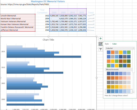
2	On the DC worksheet, select the range A4:G4, wrap the text, apply Center alignment, and apply Blue, Accent 5, Lighter 60% fill color.
3	On the DC worksheet, merge and center the title in the range A1:G1. Apply Accent5 cell style and bold to the title.
4	On the DC worksheet, change the width of column A to 34.
5	On the DC worksheet, select the range C5:F10 and insert Line Sparklines in the range G5:G10.
6	On the DC worksheet, select the range G5:G10, display the high point sparkline marker, and change the color of the high point markers to Dark Blue.
7	On the DC worksheet, select the range G5:G10, apply Same for All Sparklines for both the vertical axis minimum and maximum values.
8	On the DC worksheet, select the ranges A4:A10 and C4:F10 and create a clustered bar chart. Apply the Monochromatic color that is a blue gradient, light to dark. Apply the gradient fill to the plot area. Do not change the default gradient options.
9	Position the top-left corner of the chart in cell A13. Change the chart height to 6 inches and the chart width to 7 inches.
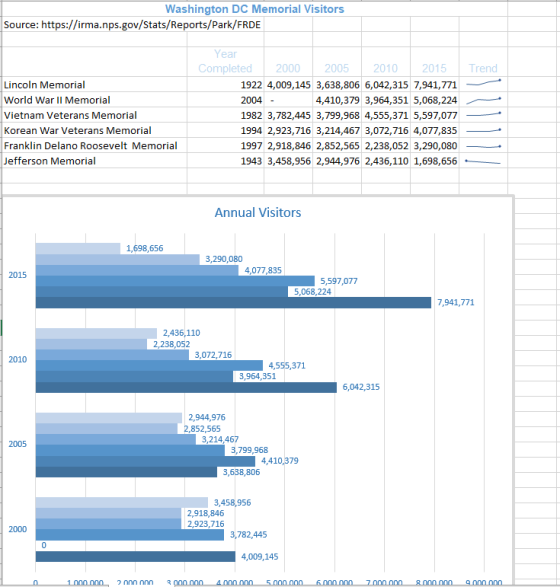
10	Change the chart title to Annual Visitors. Apply Blue, Accent 5, Darker 25% font color to the chart title and category axis labels. Change the value axis display units to Millions.
11	Apply data labels to the outside end of the 2015 data series. Apply Number format with 1 decimal place to the data labels.
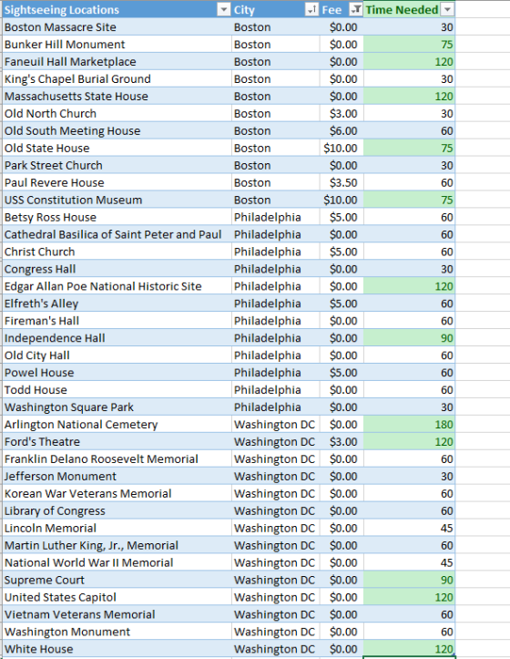
12	Click the Places sheet tab, convert the data to a table, and apply Table Style Medium 6.
13	On the Places worksheet, sort the data by City in alphabetical order and then within City, sort by Sightseeing Locations in alphabetical order.
14	On the Places worksheet, add a total row to display the average of the Time Needed column. Apply Number format with zero decimal places to the total.
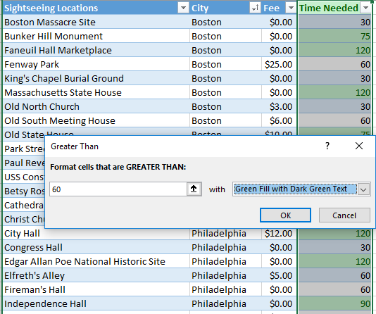
15	On the Places worksheet, select the values in the Time Needed column and apply conditional formatting to highlight cells containing values greater than 60 with Green Fill with Dark Green Text.
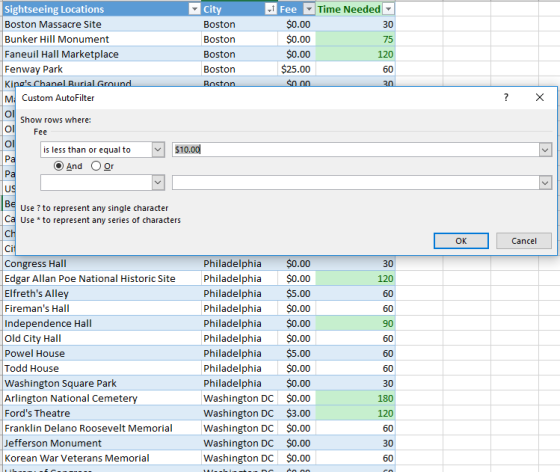
16	On the Places worksheet, apply a filter to display only fees that are less than or equal to $10.
17	On the Cities worksheet, click cell F4 and enter a formula that will subtract the Departure Date (B1) from the Return Date (B2) and then multiply the result by the Rental Car per Day value (F3).
18	On the Cities worksheet, click cell E13. Depending on the city, you will either take a shuttle to/from the airport or rent a car. Insert an IF function that compares to see if Yes or No is located in the Rental Car? Column for a city. If the city contains No, display the value in cell F2. If the city contains Yes, display the value in the Rental Car Total (F4). Copy the function from cell E13 and use the Paste Formulas option to copy the function to the range E14:E18 without removing the border in cell E18.
19	On the Cities worksheet, click cell F13. The lodging is based on a multiplier by City Type. Some cities are more expensive than others. Insert a VLOOKUP function that looks up the City Type (B13), compares it to the City/COL range (A7:B10), and returns the COL percentage. Then multiply the result of the lookup function by the Total Base Lodging (B5) to get the estimated lodging for the first city. Copy the function from cell F13 and use the Paste Formulas option to copy the function to the range F14:F18 without removing the border in cell F18.
20	On the Cities worksheet, click cell H13 and enter the function that calculates the total costs for the first city. Copy the function in cell H13 and use the Paste Formulas option to copy the function to the range H14:H18 without removing the border in cell H18.
21	On the Cities worksheet, select the range E14:H18 and apply Comma Style with zero decimal places. Select the range E13:H13 and apply Accounting Number format with zero decimal places.
22	On the Cities worksheet, in cell I2, enter a function that will calculate the average total cost per city. In cell I3, enter a function that will identify the lowest total cost. In cell I4 enter a function that will return the highest total cost.
23	On the Cities worksheet, select Landscape orientation, set a 1-inch top margin, and center the worksheet data horizontally on the page.
24	Ensure that the worksheets are correctly named and placed in the following order in the workbook: DC, Places, Cities. Save the workbook. Close the workbook and then exit Excel. Submit the workbook as directed.

Answer 1

Note: Hi, I have done all the 24 points, but point 8 and point 14 are explained well. Please check.

In the following Question, 3 worksheets are taken, 1^st worksheet named DC solves 1-11 Questions. Now, Consider the following worksheet DC:

Washington DC Memorial Visitors Source https://irma.nps.gov/Stats/Reports/ Park FRDE Year Completed 2005 1922 4.009.145 3,638,806 4,410,379 198200%) 3.782.445 3.799.968 199400%) 2.923.716 3.214.467 2000 2010 2015 Trend Lincoln Memorial World War Il Memorial Vietnam Veterans Memorial Korean War Veterans Memorial Franklin Delano Roosevelt Memorial Jefferson Memorial 6.042 315 7,941,771 3.964.351 5.068,224 4.555.371 5.597,077 3,072,716 4,077,835 2004 19970090| 2.918.846| 2.852.565 2,238,052 3,290,080 194300%) 3.458.956 2.944.976 2.436.110 1.698,656

1. Copy and paste the excel sheet. Save the excel sheet by exploring_ecap_grader_a1.xlsx.
2. Select the range A4:G4, click home tab, now choose wrap text, then apply center alignment from the same Alignment. Now, from font icon set the font color to Accent 5 Blue 60% lighter (9^th Column, 3^rd Row).
3. Select the range from A1:G1, from font icon set the font color to Accent 5 and click on Bold. Click on Merge & Center.
4. Select the column A, either change the width from the column names to 34 or choose view tab, from the workbook Views choose Page Layout and increase the width to 34.
5. Select the range G5:G10, click on insert tab, choose Sparkline Group click on Line. Now, in the data set the range from C5:F10 and set the Location range as G5:G10.
6. Select the range G5:G10, from the Design tab, choose Marker Color à High Point à Dark Blue.
7. Select the range G5:G10, from the Design tab, choose Group à Axis à Same for all Sparkline from Minimum and also choose same for all Sparkline’s from Maximum.
8. Select the data from C5:F10, click on insert tab choose clustered bar chart. Then set the Y-Axis by the range C4:F4 and X-axis as A4:A10. Now select the chart, from the top right corner, choose chart style, choose color tab and then select Monochromatic from dark Blue to light in 5^th Row. Consider the following figure:

Washington DC Memorial Visitors Source: https://irma.nps.gov/Stats/Reports/Park/FRDE Year Completed2000 2005 2010 2015 Trend Lincoln Memorial World War II Memorial Vietnam Veterans Memorial Korean War Veterans Memorial Franklin Delano Roosevelt Memorial Jefferson Memorial 1922| 4,009,145 3,638,806 6,042,315 7,941,771| 2004 1982 3,782,445 3,799,968 4,555,371 5,597,077 1994 2,923,716 3,214,467 3,072,716 4,077,835 1997 2,918,846 2,852,565 2,238,052 3,290,080 4,410,379 3,964,351 5,068,224 Chart Title Style Color Colorful 2015 2010 Monochromatic 2005 How do l change these colors? 2000

9. Now select the chart and move to the cell A13, to resize the chart click on Format tab à Size à Set Height 6 and width 7.

10. Select the chart title, now edit the text and replace the text with Annual Visitors. Now Select the complete Annual Visitors text and right click choose Font option, set the font color to Blue, Accent 5, Darker 25%. Repeat the same process for Category label axis. Now, select the value range and from the right change its value max to millions.

11. Select the chart, click on the + symbol from the top right corner of the chart. Now, Choose Data Labels from the list. Consider the following figure:

1 Chart Elements Annual Visitors Axes Axis Titles Chart Title Data Labels Data Table Error Bars Gridlines Legend Trendline 1,698,656 3,290,080 4,077,835 2015 5597 p77 5,068,224 7,941,771 2,436,110 2,238,052 3,072,716 2010 4,555,371 3,964,351 6,042,315 2,944,976 2,852,565 3,214,467 2005 3,799,968 4,410,379 3,638,806 3,458,956 2,918,846 2,923,716 2000 3,782,445 4,009,145 1,000,000 2,000,000 3,000,000 4,000,000 5,000,000 6,000,000 7,000,000 8,000,000 9,000,000 Jefferson Memorial Franklin Delano Roosevelt Memorial Korean War Veterans Memorial Vietnam Veterans Memorial World War II Memorial Lincoln Memorial

Final Worksheet of DC is as follows:

Washington DC Memorial Visitors Source: https://irma.nps.gov/Stats/Reports/Park/FRDE Year Completed 2000 2005 2010 201 5 Trend Lincoln Memorial World War II Memorial Vietnam Veterans Memorial Korean War Veterans Memorial Franklin Delano Roosevelt Memorial efferson Memorial 1922 4,009,145 3,638,806 6,042,315 7,941,771 2004- 1982 3,782,445 3,799,968 4,555,371 5,597,077 1994 2,923,716 3,214,467 3,072,716 4,077,835 1997 2,918,846 2,852,565 2,238,052 3,290,080 1943 3,458,956 2,944,976 2,436,110 1,698,656 4,410,379 3,964,351 5,068,224 Annual Visitors 1,698,656 3,290,080 4,077,835 2015 5,597,077 5,068,224 7,941,771 2,436,110 2,238,052 3,072,716 2010 4,555,371 3,964,351 6,042,315 2,944,976 2,852,565 3,214,467 2005 3,799,968 4,410,379 3,638,806 3,458,956 2,918,846 2,923,716 2000 3,782,445 4,009,145

Now Solve Steps 12 to 16, by using Places Worksheet. Consider the following Worksheet Places:

Sightseeing Locations King's Chapel Burial Ground Park Street Church Faneuil Hall Marketplace Fenway Park Old State House Old South Meeting House USS Constitution Museum Boston Massacre Site Bunker Hill Monument Paul Revere House Massachusetts State House Old North Church Edgar Allan Poe National Historic Site Time Needed City Boston Boston Boston Boston Boston Boston Boston Boston Boston Boston Boston Boston Philadelphia Philadelphia Philadelphia Philadelphia Philadelphia Philadelphia Philadelphia Philadelphia Philadelphia Philadelphia Philadelphia Philadelphia Philadelphia Washington DC $0.00 Washington DC $0.00 Washington DC $0.00 Washington DC $0.00 Washington DC $0.00 Washington DC $0.00 Washington DC $0.00 Washington DC $0.00 Washington DC $0.00 Washington DC $0.00 Washington DC $0.00 Washington DC $3.00 Fee $0.00 $25.00 $10.00 75 $10.00 $0.00 75 75 $3.50 $3.00 $12.00 City Hall Fireman's Hall Powel House Old City Hall Cathedral Basilica of Saint Peter and Paul Elfreth's Alley Christ Church Washington Square Park Congress Hall Independence Hall Betsy Ross House Todd House White House Vietnam Veterans Memorial Korean War Veterans Memorial Washington Monument Martin Luther King, Jr., Memorial Arlington National Cemetery Franklin Delano Roosevelt Memorial National World War II Memorial Jefferson Monument United States Capitol Library of Congress Ford's Theatre $0.00 180

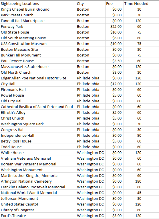
12. Click the Places sheet tab, select all the data, from the Home tab, choose Table Style Medium 6 from Format as Table from Styles.

13. Choose city column and click on Home tab à Sort and Filter from Editing. Now Select the column Sightseeing Locations and click on Re-apply to sort alphabetically based on city.

14. Insert a new row at the bottom. To calculate the average of time needed set the following formula: =AVERAGE(D2:D40). Click Enter. Now, select the cell and right click à choose Format Cells à Number à Set Decimal Places à 0.

15. Select the column Time Needed à Choose Conditional Formatting from Home Tab. Choose greater than option à Set the value as $60 and set the color with Green Fill with Dark Green Text.

Sightseeing Locations Boston Massacre Site Bunker Hill Monument Faneuil Hall Marketplace Fenway Parlk King's Chapel Burial Ground Massachusetts State House Old North Church Old South Meeting House Old State Wouco Park Stre Greater Than Paul Rev USS Cons Betsy Ros 60 Cathedra Christ Ch City Hall Congress Hall Edgar Allan Poe National Historic Site Elfreth's Alley Fireman's Hall Independence Hall city Boston Boston Boston Boston Boston Boston Boston Boston Fee ▼ Time Needed $0.00 $0.00 選),(X) $25.00 30 75 120 60 30 120 30 60 $0.00 $6.00 Format cells that are GREATER THAN: ' with Green Fill with Dark Green Text . OK Philadelphia $12.00 Philadelphia $0.00 $0.00 Philadelphia $5.00 Philtlelphia o.i Philadelphia $0.00 Cancel 120 30 120 Philadelphia 60 90

16. Select the column fees, Choose Sort & Filter à Number à Less than or equal to à $10 à OK.

Sightseeing Locations Boston Massacre Site Bunker Hill Monument Faneuil Hall Marketplace Fenway Park Ki M Custom AutoFilter city Boston Boston Boston Boston ▼ Time Needed ▼ 30 75 Fee $0.00 $0.00 $0.00 $25.00 Show rows where: Fee is less than or equal to And O $10.00 Use? to represent any single character Use * to represent any series of characters OK Cancel Ci Congress Hall Edgar Allan Poe National Historic Site Elfreth's Alle Fireman's Hall Independence Hall Old City Hall Powel House Todd House Washington Square Park Arlington National Cemeteny Ford's Theatre Franklin Delano Roosevelt Memorial Jefferson Monument Korean War Veterans Memorial Philadelphia $0.00 Philadelphia Philadelphia $5.00 Philadelphia $0.00 Philadelphia $0.00 Philadelphia $0.00 Philadelphia $5.00 Philadelphia $0.00 Philadelphia $0.00 Washington DC $0.00 Washington DC $3.00 Washington DC $0.00 Washington DC $0.00 Washington DC $0.00 $0.00 30 180 30

Consider the final worksheet after modification:

T Time Needed Sightseeing Locations Boston Massacre Site Bunker Hill Monument Faneuil Hall Marketplace King's Chapel Burial Ground Massachusetts State House Old North Church Old South Meeting House Old State House Park Street Church Paul Revere House USS Constitution Museum Betsy Ross House Cathedral Basilica of Saint Peter and Paul Christ Church Congress Hall Edgar Allan Poe National Historic Site Elfreth's Alle Fireman's Hall Independence Hall Old City Hall Powel House Todd House Washington Square Park Arlington National Cemeteny Ford's Theatre Franklin Delano Roosevelt Memorial Jefferson Monument Korean War Veterans Memorial Library of Congress Lincoln Memorial Martin Luther King, Jr., Memorial National World War II Memorial Supreme Court United States Capitol Vietnam Veterans Memorial Washington Monument White House $0.00 $0.00 $0.00 $0.00 $0.00 $3.00 $6.00 $10.00 $0.00 $3.50 $10.00 $5.00 $0.00 Boston Boston Boston Boston Boston Boston Boston Boston Boston Boston Boston Philadelphia Philadelphia Philadelphia $5.00 Philadelphia $0.00 Philadelphia Philadelphia $5.00 Philadelphia $0.00 Philadelphia $0.00 Philadelphia $0.00 Philadelphia $5.00 Philadelphia $0.00 Philadelphia $0.00 Washington DC $0.00 Washington DC $3.00 Washington DC $0.00 Washington DC $0.00 Washington DC $0.00 Washington DC $0.00 Washington DC $0.00 Washington DC $0.00 Washington DC $0.00 Washington DC $0.00 Washington DC $0.00 Washington DC $0.00 Washington DC $0.00 Washington DC $0.00 30 75 30 30 75 75 $0.00 30 180 45 45 120

Now Solve Steps 17 to 23, by using Cities Worksheet. Consider the following Worksheet Cities:

Summary Trip Costs Ground Departure Date 8/18/2018 Transportatio Round-trip Shuttle Rental Car per Day 50 Average Return Date 8/23/2018 Lowest Highest 30 Rental Car Total Lodging Base/NightS Total Base Lod Ci 115 575 COL 95% 110% 125% 140% 2 4 Shuttle or Lodging Rental Total Meals Cost Rental Car? Airfare 3 No 2 Yes 1 Yes 3 No City Type Destination City Boston Miami Orlando Philadelphia San Antonio S 367 392 299 479 218 469 375 330 285 375 285 420 Yes 4 No Washington DC

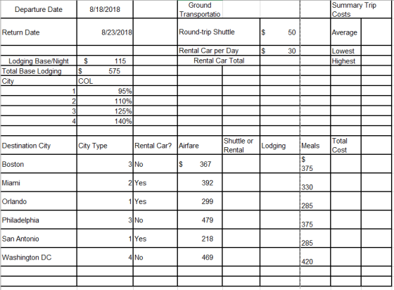
17. Click the cell F4, paste the following formula: =PRODUCT(DATEDIF(B1,B2,"d"),F3).

18. Click the cell E13, paste the following formula: =IF(C13="No",$F$2,$F$4). Now, extend the cell from E14:E18.

19. Click the cell F13, paste the following formula: =PRODUCT(VLOOKUP(B13,$A$7:$B$10,2,TRUE),$B$5). Now, extend the cell from F14:F18.

20. Click the cell H13, paste the following formula: =SUM(D13:G13). Now, extend the cell from H14:H18.

21. Select the range E14:H18, right click and choose cell formatting à number à click on comma separator and set decimal places to 0.

22. Click the cell I2, paste the following formula: =AVERAGE(H13:H18). Click the cell I3, paste the following formula: =MIN(H13:H18). Click the cell I4, paste the following formula: =MAX(H14:H19).

23. Select the complete data on the worksheet, choose Page Layout à Page Setup à Orientation à Landscape. Now, to set the margin, choose Page Setup à Margin à set top Margin to 1. Select the data, right click à Choose Cell Formatting à Choose Alignment tab à Set Horizontal Alignment as center. Consider the following worksheet with final data:

Summary Trip Costs Departure Date 8/18/2018 Ground Transportation Round-trip Shuttle Rental Car per Day Return Date 8/23/2018 50 Average1,477 30 150 Lowest Highest 1.199 1.744 115 575 Rental Car Total Lodging Base/Night Total Base Lodgin Ci COL 95% 110% 125% 140% 2 4 Total Meals Cost Destination City City Type Boston Miami Orlando Philadelphia San Antonio Washington DC Rental Car? Airfare Shuttle or Rental Lodging 367 392 299 479 218 469 50 150 150 50 150 50 719 633 546 719 546 805 375 1,511 330 1,505 285 1280 375 1,623 285 1199 2 Yes 1Yes 4 No 201,744

24. Now, save the workbook. Close the excel.