Question

Julie owns 100 shares of certain technology stock and is trying to decide how much her portfolio will be worth next month. The data table below shows the closing price of a share of stock at the end of each month from May 2009 until December 2010. Use the data to complete parts b-g b.) forecast the closing price for the stock at the end of January 2011 using a trend projection. c.) calculate the MAD for this forecast d.) check the presence of autocorrelation using alpha= 0.05. Identify the null and alternative hypotheses e.) determine the Durbin Watson statistic f.) identify the critical values and state the conclusion. g.) what concerns should you have using the trend projection to forecast with these data?

Answer 1

a)

The forecast using the trend projection method is obtained as follow,

The trend equation is,

Tbobit

Where,

ΣΥΣΧΣΧΣΧΥ bo ΠΣΧ) ΣΧΕ 2

ΠΣΧΥ ΣΧ ΣΥ ΣΧ n (ΣΧ )

From the data values,

	Period, X	Price, Y	X^2	Y^2	X*Y
	1	142	1	20164	142
	2	157	4	24649	314
	3	178	9	31684	534
	4	186	16	34596	744
	5	202	25	40804	1010
	6	205	36	42025	1230
	7	214	49	45796	1498
	8	228	64	51984	1824
	9	205	81	42025	1845
	10	204	100	41616	2040
	11	229	121	52441	2519
	12	251	144	63001	3012
	13	250	169	62500	3250
	14	256	196	65536	3584
	15	249	225	62001	3735
	16	232	256	53824	3712
	17	281	289	78961	4777
	18	298	324	88804	5364
	19	302	361	91204	5738
	20	304	400	92416	6080
Sum	210	4573	2870	1086031	52952

ΣΥ X2 2870 Y =4573, y2 X 210 1086031 XY 52952

4573 x 2870 210 x 52952 bo 20(2870) (210)2

bo 150.7211

20(52952) 210 x 4573 b1 20(2870) (210)2

b17.4218

The trend equation is,

T150.7211+734218

The forecast for the period 21 (January 2011) is obtained is,

T 150.7211+734218 x 21

T306.5789 307

c)

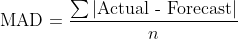
The Mean Absolute Deviation (MAD) for the forecast is obtained using the formula,

Actual Forecast MAD

	Period, X	Price, At	Forecast, Ft	|At-Ft|
	1	142	158.14	16.14
	2	157	165.56	8.56
	3	178	172.99	5.01
	4	186	180.41	5.59
	5	202	187.83	14.17
	6	205	195.25	9.75
	7	214	202.67	11.33
	8	228	210.10	17.90
	9	205	217.52	12.52
	10	204	224.94	20.94
	11	229	232.36	3.36
	12	251	239.78	11.22
	13	250	247.20	2.80
	14	256	254.63	1.37
	15	249	262.05	13.05
	16	232	269.47	37.47
	17	281	276.89	4.11
	18	298	284.31	13.69
	19	302	291.74	10.26
	20	304	299.16	4.84
Sum	210	4573	4573	224.09

$\text{MAD}=\frac{224.09}{20}=11.2043$

d)

The null and alternative hypothesis are defined as,

H0 = There is no auto correlation exists (first order). $\rho\leq 0$

H1 = Significant correlation exists (first order), $\rho> 0$

e)

The Durbin Watson test statistic is obtained using the formula,

Durbin Watson test statistic = 2-2 (Y; - Y-1)" Σ.Υ i=1

Where N = 20, Y_i is the current month's observation value and Y_i-1 is the previous month's observation value.

Period, i	Price, Yi	(Yi-Yi-1)^2	Yi2
1	142
2	157	225	24649
3	178	441	31684
4	186	64	34596
5	202	256	40804
6	205	9	42025
7	214	81	45796
8	228	196	51984
9	205	529	42025
10	204	1	41616
11	229	625	52441
12	251	484	63001
13	250	1	62500
14	256	36	65536
15	249	49	62001
16	232	289	53824
17	281	2401	78961
18	298	289	88804
19	302	16	91204
20	304	4	92416
		5996	1065867

$\text{Durbin Watson Statistic}=\frac{5996}{1065867}=0.00563$

f)

The upper and lower critical value for Durbin Watson test statistic is obtained using the Durbin Watson significance table, for k = 1, sample size, N = 20 and significance level = 0.05.

$d_\text{Upper}=1.201$

Lower 1.411

Since the Durbin Watson test statistic value is less than the lower critical value, the null hypothesis is rejected hence there is a significant positive internal association (auto correlation)

g)

Since there is a significant auto correlation exists, the assumption of trend projection of no auto correlation violated.