Question

​Altitude, x For the following data (a) display the data in a scatter plot, (b) calculate the sample correlation coefficient r, and (c) make a conclusion about the type of correlation. Use technology The altitudes (in thousands of feet) and speeds of sound (in feet per second) at these altitudes are shown in the data set below. 囲Click the icon to view the data set. (a) Display the data in a scatter plot. Choose the correct graph below OA. 1140 1140 940 1140 Speed of sound (fis) Altitude (1000's ft) Altitude (1000's ft) Data Table (b) Calculate the sample correlation coefficientr r(Round to three decimal places as needed.) (c) Make a conclusion about the type of correlation The correlation is a Altitude, X Speed of sound, y 1116.4 1097.5 1075.7 1055.6 1036.8 1016.9 994.6 969.7 968.8 968.8 968.8 linear correlation 10 15 20 25 30 35 40 45 50 Click to select your answer(s)	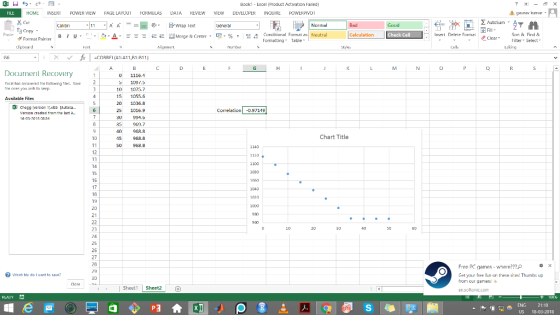Speed of​ sound, y
00	1116.41116.4
55	1097.51097.5
1010	1075.71075.7
1515	1055.61055.6
2020	1036.81036.8
2525	1016.91016.9
3030	994.6994.6
3535	969.7969.7
4040	968.8968.8
4545	968.8968.8
5050	968.8968.8

Answer 1

(a) D is the plot you should select

(b) -0.971

(c) inverse linear relation

Book1 Excel (Product Activation Failed) garav lamarP HILE HOME INSERT POWER VIEW PAGE LAYOUTFORMULAS DATA REVIEW VE DEVELOPER INQUIRE POWERPIWO 義Cut AutoSum A Arap lext libri Nuririal Bad Paste % , .。.® Conditional Format as Calculation Check Cell Insert Delete Foriat Sort &Find & ierSelect Format Painter Clear Fomatting Table Ldiirg XVfCORRFI (A1:A11,R1:R11) Documerl Recovery 0 1116.1 510A.S 10 1075.7 15 1055.6 20 1036.B 251016.9 3U 4.6 35 909.7 40 968.8 Excฝ has recovered the folowing Iles. the ores you wish to kefp Available Files 咖cregg:neroon 11.dsb [utosa.. Correlation -0.97149 Version created trom tne last A 6-03-2018 Chart Title 958. 23 26 Free PC games where???O Get yaur free fu o these sites Thambs up from our gamers! Which hla da I want to save? |Sheet1|Sheet2 ④ ENG 21:10 US 18-03-2018