Question

The daily changes in stock prices exhibit a random behavior, which means that these daily changes are independent of each other and can be approximated by a normal distribution. To test this theory, collect data for one company that is traded on the Tokyo Stock Exchange, one company traded on the Shanghai Stock Exchange, and one company traded on the Hong Kong Stock Exchange and then do the following:

1.            Record the daily closing stock price of each of these companies for six consecutive weeks (so you may have 30 values per company).

2.            For each of your six data sets, decide if the data are approximately normally distributed by:

a.            constructing the stem-and-leaf display, histogram or polygon, and boxplot.

b.           comparing data characteristics to theoretical properties.

c.            constructing a normal probability plot.

d.           Discuss the results of (a) through (c). What can you say about your three stocks with respect to daily closing prices and daily changes in closing prices? Which, if any, of the data sets are approximately normally distributed?

Answer 1

Date	id	open_s	high_s	low_s	close_s	volume_s	open_h	high_h	low_h	close_h	volume_h
2/13/2018	1	1,077	1,077	998	999	250,700	3,798	3,818	3,724	3,730	7,767,700
2/9/2018	2	1,012	1,042	1,000	1,036	148,900	3,751	3,796	3,740	3,795	8,358,200
2/8/2018	3	1,074	1,098	1,053	1,073	123,500	3,884	3,927	3,849	3,873	7,623,900
2/7/2018	4	1,151	1,151	1,061	1,063	202,200	3,933	3,947	3,839	3,840	9,005,600
2/6/2018	5	1,088	1,139	1,003	1,074	447,500	3,831	3,831	3,723	3,810	10,651,900
2/5/2018	6	1,226	1,263	1,212	1,238	185,000	3,983	4,030	3,946	3,971	9,843,400
2/2/2018	7	1,318	1,318	1,274	1,304	84,200	3,858	3,900	3,840	3,890	5,681,300
2/1/2018	8	1,317	1,325	1,281	1,309	141,700	3,850	3,871	3,844	3,859	4,709,900
1/31/2018	9	1,268	1,322	1,251	1,293	159,900	3,890	3,890	3,817	3,826	6,285,000
1/30/2018	10	1,308	1,315	1,271	1,289	202,600	3,958	3,985	3,916	3,925	3,991,000
1/29/2018	11	1,324	1,328	1,294	1,312	120,600	3,922	3,976	3,899	3,947	3,107,900
1/26/2018	12	1,269	1,313	1,262	1,308	188,000	3,950	3,968	3,931	3,933	3,316,700
1/25/2018	13	1,258	1,260	1,228	1,253	111,300	3,943	3,953	3,925	3,942	4,274,900
1/24/2018	14	1,275	1,279	1,240	1,264	123,700	4,025	4,031	3,993	3,994	2,881,200
1/23/2018	15	1,265	1,284	1,249	1,282	142,800	3,993	4,066	3,991	4,052	3,664,800
1/22/2018	16	1,216	1,256	1,196	1,247	120,800	4,000	4,000	3,960	3,980	2,830,500
1/19/2018	17	1,226	1,235	1,200	1,216	95,300	3,993	4,017	3,981	4,003	2,991,300
1/18/2018	18	1,245	1,264	1,217	1,218	182,600	4,037	4,043	3,971	3,977	4,732,000
1/17/2018	19	1,176	1,234	1,165	1,221	178,200	3,989	4,019	3,977	4,019	3,653,300
1/16/2018	20	1,169	1,207	1,151	1,200	134,500	3,983	3,998	3,965	3,989	2,983,200
1/15/2018	21	1,170	1,178	1,147	1,171	118,400	4,000	4,006	3,971	3,981	2,975,900
1/12/2018	22	1,186	1,192	1,156	1,164	100,000	4,005	4,010	3,966	3,968	5,005,900
1/11/2018	23	1,199	1,199	1,167	1,181	121,000	4,035	4,055	3,998	4,026	4,031,200
1/10/2018	24	1,217	1,219	1,179	1,211	169,500	4,035	4,151	4,028	4,102	4,692,400
1/9/2018	25	1,194	1,218	1,183	1,216	139,000	4,042	4,057	3,997	4,010	3,447,000
1/5/2018	26	1,185	1,190	1,167	1,182	53,200	4,000	4,054	3,990	4,021	4,765,200
1/4/2018	27	1,151	1,184	1,146	1,178	100,500	3,925	3,986	3,906	3,986	4,962,300
12/29/2017	28	1,155	1,161	1,131	1,137	87,700	3,860	3,880	3,852	3,862	2,100,400
12/28/2017	29	1,194	1,194	1,148	1,151	137,600	3,893	3,903	3,861	3,866	1,770,100
12/27/2017	30	1,145	1,194	1,143	1,194	102,600	3,886	3,908	3,879	3,895	1,387,100

Here, open_s, high_s, low_s, close_s, & volume_s represents the variables of the stock prices of Suzuki co. ltd. whereas open_h, high_h, low_h, close_h & volume_h represents the variables of stock prices of Honda motor co. ltd.

1) Just look at the 6th and 11th columns. close_s and close_h.  

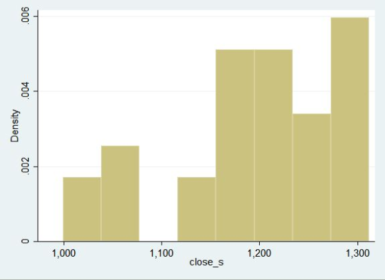
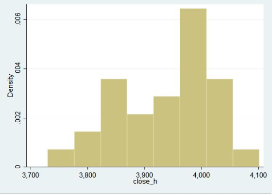
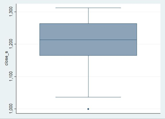
2) Now we make the stem and leaf display, histogram and boxplot of closing stock price.

Stem-and-leat plot for elose s (elose ) 9**99 10** 10* 36 10** 10**63,73,74 10** 1137 11** 51 11 64,71,78 11**81,82,94 12** 00,11,16,16,18 12** 21,38 1247,53 12** 64 12 82,89,93 13** 04,08,09,12

Stem-and-leaf plot for close h (close h) 30 37** 37** 37** 37** *10 38** 38**26 38** 38**62,66,73 38** 39** 39**25.33 39**42,47 39**68,71,77 39**80,81,86,89,94 40** 03,10,19 40**21,2 40**52 40** 40** 41**02 40,59 90,95

CN 1,000 1,100 1,200 1,300 close s

UD 3,700 3,900 close h 4,100 ei 3,800 4,000

close s 1,000 1,100 1,200 1,300

close h 3,700 3,800 3,900 4,000 4,100

b.) Various descriptive information

Variable	Obs	Mean	Std. Dev.	Min	Max
open_s	30	1202	77	1012	1324
high_s	30	1221	75	1042	1328
low_s	30	1172	83	998	1294
close_s	30	1199	85	999	1312
volume_s	30	149117	70460	53200	447500
open_h	30	3942	77	3751	4042
high_h	30	3969	83	3796	4151
low_h	30	3909	85	3723	4028
close_h	30	3936	86	3730	4102
volume_h	30	4783040	2395922	1387100	10700000

Normal F[(close_s-m)/s] 0.50 3 0.00 0.25 0.75 1.00 2 0 3

Normal F[(close h-m)/s] 0.50 6 9 0.00 0.25 0.75 1.00 3 0 2 0 3

We will test for normality by Shapiro-Wilk test.

Shapiro-Wilk W test for normal data Variable Obs Prob>z close h 30 0.96913 0.981 -0.039 0.51567 swilk close s Shapiro-Wilk W test for normal data Variable Obs Prob>z close s 30 0.93543 2·052 1.487 0.06857

In the shapirowilk test, null hypothesis state that data is normally distributed. Here, p-value for close_h is 0.515 and for close_h it is 0.068. We fail to reject the null hypothesis. Here, we observed that close_h(onda) and close_s(uzuki) are normally distributed. Thus, we found that both the variables close_h and close_s are normally distributed.