
Homework Answers
The regression model that is to be estimated is

where 
the estimated regression equation is

a) Using this
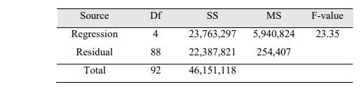
We know
k=4 is the number of independent variables
Sum of square Error (residuals), SSE = 22,387,821
degrees of freedom residuals = n-k-1 = 88
Sum of square Total (residuals), SST = 46,151,118
degrees of freedom total is n-1 = 92
The adjusted R-square is

ans: The adjusted R-square is 0.4929
b) We want to test the following hypotheses


The test statistics is F=23.35 with numerator df=4 and denominator df=88
Using F table for alpha=0.05 and numerator df=4 and denominator df=120 (The closest we can get to 88) we get the critical value of F = 2.45
We will reject the null hypothesis if the test statistics is greater than the critical value.
Here the test statistics is 23.35 and it is greater than the critical value, 2.45. Hence we reject the null hypothesis.
We conclude that the overall model is significant
c) There would be positive linear relationship between salary
and experience if the slope coefficient 
That is we want to test the following hypotheses

This is a right tailed test (the alternative hypothesis has ">").
The hypothesized value of 

Using the following
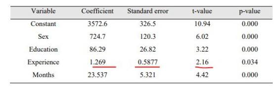
the test statistics is

The degrees of freedom for t statistics is n-k-1=88
The p-value given in the output is 0.034 is for a 2 tailed test. For one tailed test the p-value is half of that, that is p-value=0.034/2=0.017
We will reject the null hypothesis if the p-value is less than level of significance
Here the p-value is 0.017 and it is less than 0.05 level of significance. Hence we reject the null hypothesis.
We conclude that there is a positive linear relationship between Salary and Experience, after accounting for the effect of the variables, Sex, Education, and Months
d) the predicted salary for Sex=1 (man), Education = 15, Experience = 20 , months=10 is

ans: The salary for a man with 15 years of education, 20 months of experience and 10 months with in the company is $5,852.4
(Important: In the question pasted, the unit of the salary is not given. Please express the figure 5,852.4 accordingly)
e) To know if there is an interaction between Sex and Experience we will modify the model as below

If the interaction is significant it means that the coefficient

The salary model for a man is (by setting Sex=1)

The salary model for a woman (by setting sex=0) is

It means that the predicted salary changes by 

Add Answer to:
3. The table below shows the regression output of a multiple regression model relating the beginn...
Consider the following ANOVA table for a multiple regression model. Complete parts a through e be...
 *ANSWERS IN BOX ARE INCORRECT*
Consider the following ANOVA table for a multiple regression model. Complete parts a through e below. Source Regression 3 3,600 1200 20 Residual 35 2,100 60 Total df SSMSF 38 5,700 a. What is the size of this sample? n41 b. How many independent variables are in this model? c. Calculate the multiple coefficient of determination. R0.5882 Round to four decimal places as needed.) d. Test the significance of the overall regression model using α=0.05...
*ANSWERS IN BOX ARE INCORRECT*
Consider the following ANOVA table for a multiple regression model. Complete parts a through e below. Source Regression 3 3,600 1200 20 Residual 35 2,100 60 Total df SSMSF 38 5,700 a. What is the size of this sample? n41 b. How many independent variables are in this model? c. Calculate the multiple coefficient of determination. R0.5882 Round to four decimal places as needed.) d. Test the significance of the overall regression model using α=0.05...
Table 2 below shows cross-sectional regression results from the study of Beck, Degryse, and Kneer...
 Table 2 below shows cross-sectional regression results from the study of Beck, Degryse, and Kneer (2014).1 The dependent variable is the economic growth (GDP per capita growth) of different countries averaged over the period 1980- 2007. The explanatory variables are defined as follows: intermediation is a proxy for the size of financial sector and equal to the logarithm of the credit over GDP for every country in the sample; initial GDP is the logarithm of the GDP per capita in...
 *ANSWERS IN BOX ARE INCORRECT*
Consider the following ANOVA table for a multiple regression model. Complete parts a through e below. Source Regression 3 3,600 1200 20 Residual 35 2,100 60 Total df SSMSF 38 5,700 a. What is the size of this sample? n41 b. How many independent variables are in this model? c. Calculate the multiple coefficient of determination. R0.5882 Round to four decimal places as needed.) d. Test the significance of the overall regression model using α=0.05...
*ANSWERS IN BOX ARE INCORRECT*
Consider the following ANOVA table for a multiple regression model. Complete parts a through e below. Source Regression 3 3,600 1200 20 Residual 35 2,100 60 Total df SSMSF 38 5,700 a. What is the size of this sample? n41 b. How many independent variables are in this model? c. Calculate the multiple coefficient of determination. R0.5882 Round to four decimal places as needed.) d. Test the significance of the overall regression model using α=0.05...
 Table 2 below shows cross-sectional regression results from the study of Beck, Degryse, and Kneer (2014).1 The dependent variable is the economic growth (GDP per capita growth) of different countries averaged over the period 1980- 2007. The explanatory variables are defined as follows: intermediation is a proxy for the size of financial sector and equal to the logarithm of the credit over GDP for every country in the sample; initial GDP is the logarithm of the GDP per capita in...
Most questions answered within 3 hours.
-
In a recent survey of homes in a major Midwestern city, 10% of
the homes have...
asked 33 seconds from now -
T F 3. The existence of financial markets is required to have
interest rates in a...
asked 6 minutes ago -
Write in c++ please
Read and write 5 students information such as, Student
ID, first name,...
asked 7 minutes ago -
Compare/Contrast the Lac and Ara operons.
asked 7 minutes ago -
information was collected by an extensive marketing project that
lasted over the past 12 years and...
asked 7 minutes ago -
Part A
What is the maximum speed with which a 1200-kg car can round a
turn...
asked 9 minutes ago -
A. Compare the characteristics of job costing and
process costing. Consider how each method impacts the...
asked 8 minutes ago -
4. An elderly person's range of vision is between 70 cm and 300
cm from the...
asked 11 minutes ago -
Suppose that 1 kg of water, initially at 350 K, is turned into
steam at 373...
asked 18 minutes ago -
Equilibrium in the Keynesian model requires that withdrawals be
the same as:
asked 18 minutes ago -
What is the difference between apoptosis and necrosis?
(b) What is the role of apoptosis in...
asked 28 minutes ago -
A galaxy is a large grouping of stars. Approximately how many
stars are in the Milky...
asked 1 hour ago