Question

Consider polynomial interpolation of the function f(x)=1/(1+25x^2) on the interval [-1,1] by (1) an interpolating polynomial determined by m equidistant interpolation points, (2) an interpolating polynomial determined by interpolation at the m zeros of the Chebyshev polynomial T_m(x), and (3) by interpolating by cubic splines instead of by a polynomial. Estimate the approximation error by evaluation max_i |f(z_i)-p(z_i)| for many points z_i on [-1,1]. For instance, you could use 10m points z_i. The cubic spline interpolant can be determined in MATLAB; see "help spline". Use m=10 and m=20. Compute splines that interpolate at equidistant nodes and at Chebyshev nodes. Provide tables of the errors and plots of the function f and the interpolating polynomials and splines.

Answer 1

Matlab function for Lagrange Interpolation clear all close all %first function %loop for Lagrange polynomial for all n for n-10:10:20 k-k+1i %Equidistance data points x1-linspace (a,b, n); yl-double(fl (x1))i; Chebyshev data points for i-1:n x2 (i)- (1/2)(a+b)+(1/2)(b-a)*cos(((2*i-1) *pi) (2 n)) end y2-double (fl (x1)) 8x1-independent variable;y1-dependent variable;x-value at which we have to %find the dependent variable ;y-corresponding value of dependent variable at x pl-polyfit (xl,yl,n-1); p2-polyfit (x2,y2,n-1); %the interpolated data polyfit xx1-linspace (a,b,200) polynomial fit for Equidistance points yyl-polyval(pl,xxl); polynomial fit for Chebyshev points yy2-polyval (p2, xxl); %cubic spline yy3_eq-spline (xl,yl, xxl); yy3.ch-spline ( x2 , у 2 , xx 1 ) ; plotting of function figure(k) hold on plot (xxl,yyl, 'Linewidth',2) plot (xx1,yy2, 'Linewidth',2) plot (xxl,yy3_eq, Linewidth', 2) plot (xxl,yy3_ch, Linewidth',2) plot (xxl,fl (xxl), 'Linewidth',2) xlabel(x ylabel'f(x) ) legend Equidistance', 'Chebyshev, "Spline equidistance', Spline equidistance, Actual')

n',n,norm (yyl-fl (xxl))) n',n,norm (yy2-f1 (xx1))) is %e .\n',n,norm(yy3_eq-f1(xx 1))) e. Inin,n, norm(yy3_ch-fl (xxl))) title( sprintf('Interpolating polynonial for n-%d.,n)) fprint f (.\tError in Equidistance interpolation for n-%d is %e. fprintf'tError in Chebyshev interpolation for n-d is se fprintf tError in Equidistance spline interpolation for n-sd fprint f ( "\tError in Chebyshev spline interpolation for n#d is end 88888888888888888888 End of code 8888888888888888888 8- Error in Equidistance interpolation for n-10 is 1.546059e+0o. Error in Chebyshev interpolation for n-10 is 1.568430e+00. Error in Equidistance spline interpolation for n-10 is 5.777008e-01 Error in Chebyshev spline interpolation for n-io is 1.600577e+00. Error in Equidistance interpolation for n-20 is 2.507453e+01 Error in Chebyshev interpolation for n=20 is 1.553537e+00. Error in Equidistance spline interpolation for n=20 is 3.705715e-02. Error in Chebyshev spline interpolation for n-20 is 1.559637e+00

Interpolating polynomial for n-10 Equidistance Chebyshev Spline equidistance Spline equidistance 0.8 -Actual 0.6 0.4 0.2 -0.2 -0.4 -0.8 -0.60.4 0.2 02 04 0.6 0.8 Interpolating polynomial for n- 20 Equidistance Spline equidistance Spline equidistance Actual -0.8 0.2 02 0.4 0.6 0.8

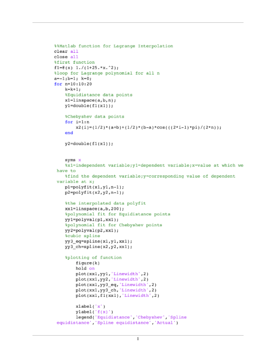
%%Matlab function for Lagrange Interpolation
clear all
close all
%first function
f1=@(x) 1./(1+25.*x.^2);
%loop for Lagrange polynomial for all n
a=-1;b=1; k=0;
for n=10:10:20
    k=k+1;
    %Equidistance data points
    x1=linspace(a,b,n);
    y1=double(f1(x1));
  
    %Chebyshev data points
    for i=1:n
        x2(i)=(1/2)*(a+b)+(1/2)*(b-a)*cos(((2*i-1)*pi)/(2*n));
    end

    y2=double(f1(x1));
  
  
    syms x
    %x1=independent variable;y1=dependent variable;x=value at which we have to
    %find the dependent variable;y=corresponding value of dependent variable at x;
    p1=polyfit(x1,y1,n-1);
    p2=polyfit(x2,y2,n-1);
  
    %the interpolated data polyfit
    xx1=linspace(a,b,200);
    %polynomial fit for Equidistance points
    yy1=polyval(p1,xx1);
    %polynomial fit for Chebyshev points
    yy2=polyval(p2,xx1);
    %cubic spline
    yy3_eq=spline(x1,y1,xx1);
    yy3_ch=spline(x2,y2,xx1);
  
    %plotting of function
        figure(k)
        hold on
        plot(xx1,yy1,'Linewidth',2)
        plot(xx1,yy2,'Linewidth',2)
        plot(xx1,yy3_eq,'Linewidth',2)
        plot(xx1,yy3_ch,'Linewidth',2)
        plot(xx1,f1(xx1),'Linewidth',2)
      
        xlabel('x')
        ylabel('f(x)')
        legend('Equidistance','Chebyshev','Spline equidistance','Spline equidistance','Actual')
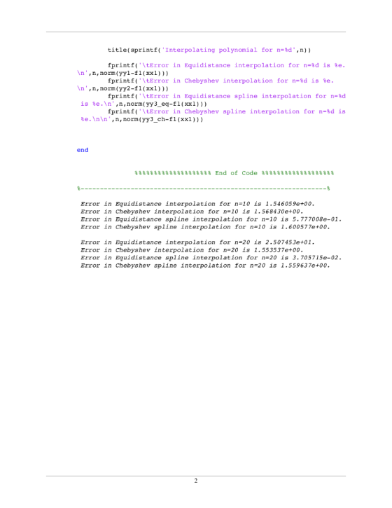
        title(sprintf('Interpolating polynomial for n=%d',n))
  
        fprintf('\tError in Equidistance interpolation for n=%d is %e.\n',n,norm(yy1-f1(xx1)))
        fprintf('\tError in Chebyshev interpolation for n=%d is %e.\n',n,norm(yy2-f1(xx1)))
        fprintf('\tError in Equidistance spline interpolation for n=%d is %e.\n',n,norm(yy3_eq-f1(xx1)))
        fprintf('\tError in Chebyshev spline interpolation for n=%d is %e.\n\n',n,norm(yy3_ch-f1(xx1)))
      

end

               %%%%%%%%%%%%%%%%%%%% End of Code %%%%%%%%%%%%%%%%%%%

%----------------------------------------------------------------%