
Homework Answers
| Data Entered | ||||
| Col 1 | Col 2 | Col 3 | Col 4 | |
| Row 1 | 5.2 5.9 6.3 |
7.4 7.0 7.6 |
6.3 6.7 6.1 |
--- |
| Row 2 | 7.1 7.4 7.5 |
7.4 7.3 7.1 |
7.3 7.5 7.2 |
--- |
| Row 3 | 7.6 7.2 7.4 |
7.6 7.5 7.8 |
7.2 7.3 7.0 |
--- |
| Row 4 | 7.2 7.5 7.2 |
7.4 7.0 6.9 |
6.8 6.6 6.4 |
--- |
| Summary Data | Within each box: Item 1 = N Item 2 =  X Item
3 = Mean X Item
3 = MeanItem 4 =  X2 Item
5 = Variance X2 Item
5 = VarianceItem 6 = Std. Dev. Item 7 = Std. Err. |
||||
| C1 | C2 | C3 | C4 | Tot. | |
| R1 | 3 17.400000000000002 5.8 101.54 0.31 0.56 0.32 |
3 22 7.3333 161.52 0.09 0.31 0.18 |
3 19.1 6.3667 121.78999999999999 0.09 0.31 0.18 |
--- | 9 58.5 6.5 384.85 0.58 0.76 0.25 |
| R2 | 3 22 7.3333 161.42000000000002 0.04 0.21 0.12 |
3 21.799999999999997 7.2667 158.46 0.02 0.15 0.09 |
3 22 7.3333 161.38 0.02 0.15 0.09 |
--- | 9 65.8 7.3111 481.26 0.02 0.15 0.05 |
| R3 | 3 22.200000000000003 7.4 164.36 0.04 0.2 0.12 |
3 22.9 7.6333 174.85 0.02 0.15 0.09 |
3 21.5 7.1667 154.13 0.02 0.15 0.09 |
--- | 9 66.6 7.4 493.34 0.06 0.25 0.08 |
| R4 | 3 21.9 7.3 159.93 0.03 0.17 0.1 |
3 21.3 7.1 151.37 0.07 0.26 0.15 |
3 19.799999999999997 6.6 130.76 0.04 0.2 0.12 |
--- | 9 63 7 442.06 0.13 0.36 0.12 |
| Tot. | 12 83.5 6.9583 587.25 0.57 0.75 0.22 |
12 88 7.3333 646.2 0.08 0.28 0.08 |
12 82.4 6.8667 568.06 0.2 0.45 0.13 |
--- | 36 253.9 7.0528 1801.51 0.31 0.56 0.09 |
| ANOVA Summary | |||||
| Source | SS | df | MS | F | P |
| Rows | 4.46 | 3 | 1.49 | 21.89 | <.0001 |
| Columns | 1.47 | 2 | 0.74 | 10.82 | 0.0004 |
| r x c | 3.25 | 6 | 0.54 | 7.98 | 0.0001 |
| Error | 1.63 | 24 | 0.07 | ||
| Total | 10.81 | 35 | |||
| Critical Values for the Tukey HSD Test | |||
| HSD[.05] | HSD[.01] | HSD=the absolute [unsigned] difference between any two means (row means, column means, or cell means) required for significance at the designated level: HSD[.05] for the .05 level; HSD[.01] for the .01 level. The HSD test between row means can be meaningfully performed only if the row effect is significant; between column means, only if the column effect is significant; and between cell means, only if the interaction effect is significant. | |
| Rows [4] | 0.34 | 0.43 | |
| Columns[3] | 0.27 | 0.34 | |
| Cells[12] | 0.77 | 0.92 | |
Add Answer to:
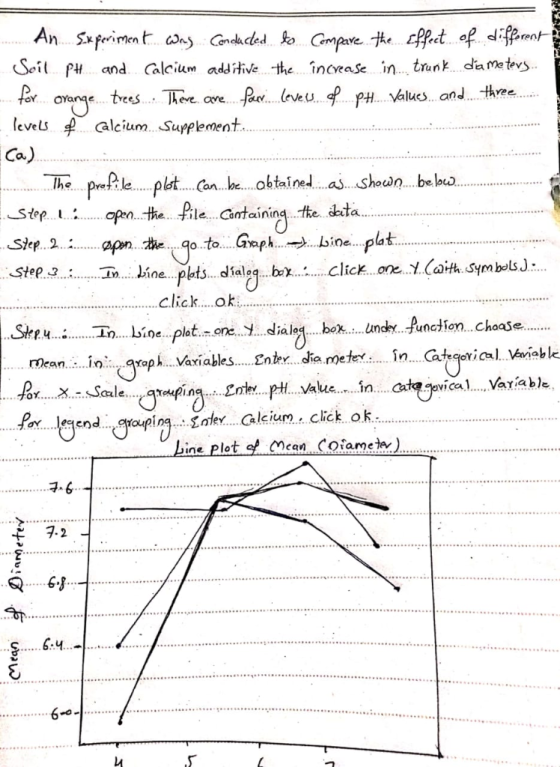
4. A n experiment was set up to compare the effect of different soil pH and calcium additives on ...
the same brand/model. The university supplier has three different models. The lab manager has borrowed one...
 the same brand/model. The university supplier has three different models. The lab manager has borrowed one of each of the three models for a week in order to test which one is the most reliable before deciding to do the purchase. A co-op student who works in the lab is assigned to test each pH meter seven times with a solution that has a known pH of 7. The plot below is the result of the pH analysis (of the...
4.3 Analysis Assignment #4 Note 1: all assignments moving forward must adhere to the appropriate Six Ste...
 4.3 Analysis Assignment #4 Note 1: all assignments moving forward must adhere to the appropriate Six Step Process (SSP). As our study materials have specified, the SSP has 3 versions. Version 1 is to be used for all t-tests; for all correlation analyses and Version 3 is be used for all regression analyses. Note 2: The data sets for Q1, Q2 and Q3 below can be downloaded here. Week 4 Analysis Assignments.xlsx Q1: (30 points) Complete the following data analysis:...
CASE 1-5 Financial Statement Ratio Computation Refer to Campbell Soup Company's financial Campbell Soup statements in...
 CASE 1-5 Financial Statement Ratio Computation Refer to Campbell Soup Company's financial Campbell Soup statements in Appendix A. Required: Compute the following ratios for Year 11. Liquidity ratios: Asset utilization ratios:* a. Current ratio n. Cash turnover b. Acid-test ratio 0. Accounts receivable turnover c. Days to sell inventory p. Inventory turnover d. Collection period 4. Working capital turnover Capital structure and solvency ratios: 1. Fixed assets turnover e. Total debt to total equity s. Total assets turnover f. Long-term...
 the same brand/model. The university supplier has three different models. The lab manager has borrowed one of each of the three models for a week in order to test which one is the most reliable before deciding to do the purchase. A co-op student who works in the lab is assigned to test each pH meter seven times with a solution that has a known pH of 7. The plot below is the result of the pH analysis (of the...
 4.3 Analysis Assignment #4 Note 1: all assignments moving forward must adhere to the appropriate Six Step Process (SSP). As our study materials have specified, the SSP has 3 versions. Version 1 is to be used for all t-tests; for all correlation analyses and Version 3 is be used for all regression analyses. Note 2: The data sets for Q1, Q2 and Q3 below can be downloaded here. Week 4 Analysis Assignments.xlsx Q1: (30 points) Complete the following data analysis:...
 CASE 1-5 Financial Statement Ratio Computation Refer to Campbell Soup Company's financial Campbell Soup statements in Appendix A. Required: Compute the following ratios for Year 11. Liquidity ratios: Asset utilization ratios:* a. Current ratio n. Cash turnover b. Acid-test ratio 0. Accounts receivable turnover c. Days to sell inventory p. Inventory turnover d. Collection period 4. Working capital turnover Capital structure and solvency ratios: 1. Fixed assets turnover e. Total debt to total equity s. Total assets turnover f. Long-term...
Most questions answered within 3 hours.
-
BASED ON THE AIRBNB, ETSY, UBER: GROWING FROM ONE THOUSAND TO
ONE MILLION CUSTOMERS HARVARD CASE:...
asked 13 minutes ago -
Which of these methods cause sterilization?
Autoclaving
Dry heat
Gamma irradiation
Ethylene oxide
A.
Yes
No...
asked 18 minutes ago -
A biologist wishes to estimate the effect of an antibiotic on
the growth of a particular...
asked 26 minutes ago -
O’Deesha Company has the following information available:
Quality engineering of
products
$20,000
Quality training of
employees &n
asked 34 minutes ago -
a) Draw two water molecules.
b) Clearly name and label the type of bond that exists...
asked 1 hour ago -
C - Language
Write a loop that sets each array element to the sum of itself...
asked 2 hours ago -
(63
#14)
which of the following statments best describes how chamging
the concentration of the substances...
asked 6 hours ago -
In the following reaction, which element is undergoing
oxidation: Na2SO3 + N2O --> N2 + Na2SO4...
asked 7 hours ago -
Which of the following pairs of ions have the same electron
configuration?
I: Br− and Se2−...
asked 9 hours ago -
The Foremost Composite Materials Company is planning a two-day
sales conference for October 19-20. The conference...
asked 10 hours ago -
3) Illustrate the observed pattern of relatedness of organisms
versus adaptations to specific conditions. This means...
asked 10 hours ago -
In winter a lake has a 0.35 m thick ice layer over 1.10 m of
water....
asked 11 hours ago