
Homework Answers

Add Answer to:
2019-Numerical Analysis- Quiz-2 1. Let f()-( (a) Use quadratic Lagrange interpolation based on th...
12 26 14 4. (15 marks) Let f(x)=/2x+1 . Use quadratic Lagrange interpolation based on the...
 12 26 14 4. (15 marks) Let f(x)=/2x+1 . Use quadratic Lagrange interpolation based on the nodes x, 0, x-1 and x, 2 to approximate f(1.2)
12 26 14 4. (15 marks) Let f(x)=/2x+1 . Use quadratic Lagrange interpolation based on the nodes x, 0, x-1 and x, 2 to approximate f(1.2)
12 26 14 4. (15 marks) Let f(x)=/2x+1 . Use quadratic Lagrange interpolation based on the nodes x, 0, x-1 and x, 2 to approximate f(1.2)
5. Write down the error term E3(x) for cubic Lagrange interpolation to f(x), where interpolation is...
 5. Write down the error term E3(x) for cubic Lagrange interpolation to f(x), where interpolation is to be exact at the four nodes xo = -1, x1 = 0, x2 = 3, and x3 = 4 and f(x) is given by (a) f(x) = 4x3 -- 3x + 2 (b) f(x)= x4 - 2x3 (c) f(x) = x3 – 5x4
5 Let f(3) = e', 0 <<< 2. Using the val e, 0 SXS 2. Using...
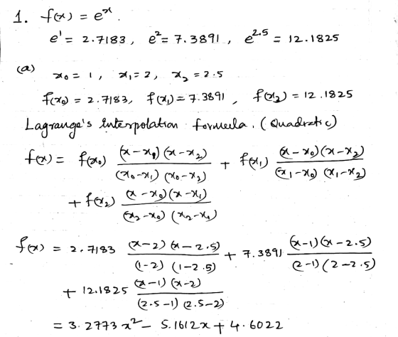
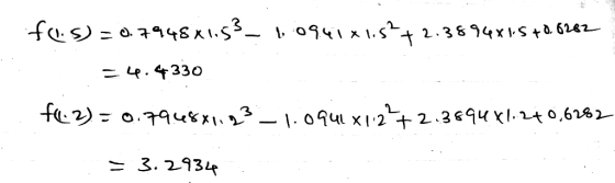
 5 Let f(3) = e', 0 <<< 2. Using the val e, 0 SXS 2. Using the values in the table below, perform the following computations x 0.0 0.5 1.0 2.0 f(x) 1.0 1.6487 2.7183 7.3890 (a) Approximate f(0.25) using linear interpolation with Xo = 0 and 21 = 0.5. (8 marks) (b) Approximate /(0.25) by using the quadratic interpolating polynomial with Xo = 0,2 = 1 and 2 = 2. [10 marks (c) Which approximations are better? Why? [2...
where x is in radians. Use Guadra tic lagrange interpolation bas ed on the nodles Xo 0.x0.5 and xz-lo to...
 where x is in radians. Use Guadra tic lagrange interpolation bas ed on the nodles Xo 0.x0.5 and xz-lo to apporimate f(os and fll.2) Construct the Divided- Difference lable basedl an the node xo 1.x- 2,X2-4and x3-t, andl find the Newton Polynomial based on xo, Xiandx xk yk 2 6 5
where x is in radians. Use Guadra tic lagrange interpolation bas ed on the nodles Xo 0.x0.5 and xz-lo to apporimate f(os and fll.2)
Construct the Divided- Difference lable...
where x is in radians. Use Guadra tic lagrange interpolation bas ed on the nodles Xo 0.x0.5 and xz-lo to apporimate f(os and fll.2) Construct the Divided- Difference lable basedl an the node xo 1.x- 2,X2-4and x3-t, andl find the Newton Polynomial based on xo, Xiandx xk yk 2 6 5
where x is in radians. Use Guadra tic lagrange interpolation bas ed on the nodles Xo 0.x0.5 and xz-lo to apporimate f(os and fll.2)
Construct the Divided- Difference lable...
Problem 5 (programming): Create a MATLAB function named lagrange interp.m to perform interpolation using Lagrange polynomials....
 Problem 5 (programming): Create a MATLAB function named lagrange interp.m to perform interpolation using Lagrange polynomials. Download the template for function lagrange interp.m. The tem Plate is in homework 4 folder utl TritonED·TIue function lakes in the data al nodex.xi and yi, as well as the target x value. The function returns the interpolated value y. Here, xi and yi are vectors while x and y are scalars. You are not required to follow the template; you can create the...
1. Consider the Runge function, f:IH 1/1+25r). (a) Use your Lagrange interpolation code (from the...
 1. Consider the Runge function, f:IH 1/1+25r). (a) Use your Lagrange interpolation code (from the previous worksheets) to approximate f using 10, 20, 30, and 40 equispaced points from -1 and 1 (inclusive). Make a (single) plot comparing these four approximations with the (exact) function f. Use a legend to help distinguish the five curves. Intuitively, increasing the number of sample points should give a 'better' approximation. Does it? (A qualitative answer is sufficient.) (b) Repeat Part (a) using piecewise...
(a). Use the numbers (called nodes) Xo = 2.0, x1 = 2.4, and x2 = 2.6...
 (a). Use the numbers (called nodes) Xo = 2.0, x1 = 2.4, and x2 = 2.6 to find the second Lagrange interpolating polynomial for f(x) = sin(In x). Using 4-digit rounding arithmatic. (b). Use this polynomial to approximate f(1). Using 4-digit rounding arithmatic.
Question 3 ( 14 Points) (a). Use the numbers (called nodes) Xo = 2.0, x1 =...
 Question 3 ( 14 Points) (a). Use the numbers (called nodes) Xo = 2.0, x1 = 2.4, and x2 = 2.6 to find the second Lagrange interpolating polynomial for f(x) = sin(In x). Using 4-digit rounding arithmatic. (b). Use this polynomial to approximate f(1). Using 4-digit rounding arithmatic.
Consider polynomial interpolation of the function f(x)=1/(1+25x^2) on the interval [-1,1] by (1) ...
Consider polynomial interpolation of the function f(x)=1/(1+25x^2) on the interval [-1,1] by (1) an interpolating polynomial determined by m equidistant interpolation points, (2) an interpolating polynomial determined by interpolation at the m zeros of the Chebyshev polynomial T_m(x), and (3) by interpolating by cubic splines instead of by a polynomial. Estimate the approximation error by evaluation max_i |f(z_i)-p(z_i)| for many points z_i on [-1,1]. For instance, you could use 10m points z_i. The cubic spline interpolant can be determined in...
this is numerical analysis 2. Consider the function f(x) = -21° +1. (a) Calculate the interpolating...
 this is numerical analysis
2. Consider the function f(x) = -21° +1. (a) Calculate the interpolating polynomial pz() for data using the nodes 2o = -1, 11 = 0, 12 = 1. Simplify the polynomial to standard form. Use the error theorem for polynomial interpolation to bound the error f(x) - P2(x) on the interval (-1,2). Is this bound realistic?
this is numerical analysis
2. Consider the function f(x) = -21° +1. (a) Calculate the interpolating polynomial pz() for data using the nodes 2o = -1, 11 = 0, 12 = 1. Simplify the polynomial to standard form. Use the error theorem for polynomial interpolation to bound the error f(x) - P2(x) on the interval (-1,2). Is this bound realistic?
 12 26 14 4. (15 marks) Let f(x)=/2x+1 . Use quadratic Lagrange interpolation based on the nodes x, 0, x-1 and x, 2 to approximate f(1.2)
12 26 14 4. (15 marks) Let f(x)=/2x+1 . Use quadratic Lagrange interpolation based on the nodes x, 0, x-1 and x, 2 to approximate f(1.2)
12 26 14 4. (15 marks) Let f(x)=/2x+1 . Use quadratic Lagrange interpolation based on the nodes x, 0, x-1 and x, 2 to approximate f(1.2)
 5. Write down the error term E3(x) for cubic Lagrange interpolation to f(x), where interpolation is to be exact at the four nodes xo = -1, x1 = 0, x2 = 3, and x3 = 4 and f(x) is given by (a) f(x) = 4x3 -- 3x + 2 (b) f(x)= x4 - 2x3 (c) f(x) = x3 – 5x4
 5 Let f(3) = e', 0 <<< 2. Using the val e, 0 SXS 2. Using the values in the table below, perform the following computations x 0.0 0.5 1.0 2.0 f(x) 1.0 1.6487 2.7183 7.3890 (a) Approximate f(0.25) using linear interpolation with Xo = 0 and 21 = 0.5. (8 marks) (b) Approximate /(0.25) by using the quadratic interpolating polynomial with Xo = 0,2 = 1 and 2 = 2. [10 marks (c) Which approximations are better? Why? [2...
 where x is in radians. Use Guadra tic lagrange interpolation bas ed on the nodles Xo 0.x0.5 and xz-lo to apporimate f(os and fll.2) Construct the Divided- Difference lable basedl an the node xo 1.x- 2,X2-4and x3-t, andl find the Newton Polynomial based on xo, Xiandx xk yk 2 6 5
where x is in radians. Use Guadra tic lagrange interpolation bas ed on the nodles Xo 0.x0.5 and xz-lo to apporimate f(os and fll.2)
Construct the Divided- Difference lable...
where x is in radians. Use Guadra tic lagrange interpolation bas ed on the nodles Xo 0.x0.5 and xz-lo to apporimate f(os and fll.2) Construct the Divided- Difference lable basedl an the node xo 1.x- 2,X2-4and x3-t, andl find the Newton Polynomial based on xo, Xiandx xk yk 2 6 5
where x is in radians. Use Guadra tic lagrange interpolation bas ed on the nodles Xo 0.x0.5 and xz-lo to apporimate f(os and fll.2)
Construct the Divided- Difference lable...
 Problem 5 (programming): Create a MATLAB function named lagrange interp.m to perform interpolation using Lagrange polynomials. Download the template for function lagrange interp.m. The tem Plate is in homework 4 folder utl TritonED·TIue function lakes in the data al nodex.xi and yi, as well as the target x value. The function returns the interpolated value y. Here, xi and yi are vectors while x and y are scalars. You are not required to follow the template; you can create the...
 1. Consider the Runge function, f:IH 1/1+25r). (a) Use your Lagrange interpolation code (from the previous worksheets) to approximate f using 10, 20, 30, and 40 equispaced points from -1 and 1 (inclusive). Make a (single) plot comparing these four approximations with the (exact) function f. Use a legend to help distinguish the five curves. Intuitively, increasing the number of sample points should give a 'better' approximation. Does it? (A qualitative answer is sufficient.) (b) Repeat Part (a) using piecewise...
 (a). Use the numbers (called nodes) Xo = 2.0, x1 = 2.4, and x2 = 2.6 to find the second Lagrange interpolating polynomial for f(x) = sin(In x). Using 4-digit rounding arithmatic. (b). Use this polynomial to approximate f(1). Using 4-digit rounding arithmatic.
 Question 3 ( 14 Points) (a). Use the numbers (called nodes) Xo = 2.0, x1 = 2.4, and x2 = 2.6 to find the second Lagrange interpolating polynomial for f(x) = sin(In x). Using 4-digit rounding arithmatic. (b). Use this polynomial to approximate f(1). Using 4-digit rounding arithmatic.
 this is numerical analysis
2. Consider the function f(x) = -21° +1. (a) Calculate the interpolating polynomial pz() for data using the nodes 2o = -1, 11 = 0, 12 = 1. Simplify the polynomial to standard form. Use the error theorem for polynomial interpolation to bound the error f(x) - P2(x) on the interval (-1,2). Is this bound realistic?
this is numerical analysis
2. Consider the function f(x) = -21° +1. (a) Calculate the interpolating polynomial pz() for data using the nodes 2o = -1, 11 = 0, 12 = 1. Simplify the polynomial to standard form. Use the error theorem for polynomial interpolation to bound the error f(x) - P2(x) on the interval (-1,2). Is this bound realistic?
Most questions answered within 3 hours.
-
Calculate the number density of argon gas at a temperature of
24C and a pressure of...
asked 3 hours ago -
Alternative
Classification
How to Estimate
Probabilities from Data? ( For continuous Attributes)
And How to generate...
asked 3 hours ago -
An explosion breaks a 20.0-kg object into three parts. The
object is initially moving at a...
asked 3 hours ago -
Calculate the approximate number of residues of Rubisco, which
is involved in carbon fixation in plants,...
asked 4 hours ago -
Other decisions about scientific claims can have a much broader
impact.ENERGYarrow-10x10.png, environment, health, security - all...
asked 5 hours ago -
I need to write a research paper and work cited about this
topic: The United States...
asked 6 hours ago -
Hello! I was wondering if I could have some help?
If the vapor pressure of carvone...
asked 6 hours ago -
An economist wants to estimate the mean per capita income (in
thousands of dollars) for a...
asked 6 hours ago -
What would be the input/output characteristic of a circuit
obtained by putting two of your 2's-complementers...
asked 6 hours ago -
In Drosophila, the transition from the syncytial blastoderm
stage to the cellular blastoderm stage is a...
asked 7 hours ago -
Project management question:
Name 3 different types of resources (hint: humans are one
type)
asked 7 hours ago -
Consider the following reaction: C 2H 2( g) + 2H 2( g) C 2H 6(
g)...
asked 7 hours ago