Question

Exercise 5.3: Consider the integral Plot of the integral from 0 to x 0.8 e: more hints You need to print E(x) with different x values. 0.6 1 Plotting the function will help The calculated values can be different depending on steps.4 Remember that this is an approximate numerical calculation. 1 1 Plot of the tunction E(x= 0.0)= 0.0 E(x= 0.1)= 0.09966764778950421 E(x = 0.2 ) = 0.197364 90282 106237 E(x = 0.3 ) = 0.2912374713875844 E(x0.4) 0.3796519307458013 E(x= 0.5)= 0.46127938390778084 E(x = 0.6 ) = 0.535151015166433 E(x= 0.7)= 0.6006821658903023 E(x0.8) 0.6576653567498664 Ex 0.9) 0.7062361099178961 E(x= 1.0)= 0.7468180014679697 2 4 7 0.0 3.0 0.5 1.0 1.5 2.0 2.5 0.5 3.0

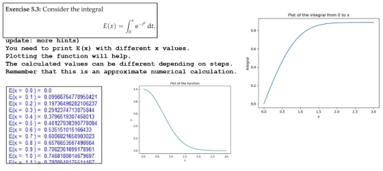
Evaluate the integral for values of x from 0 to 3 in steps of 0.1 AND plot the integral.

The program needs to be written in Python 3. Can only import numpy and matplotlib. CAN NOT use lambda functions or classes of any kind.

Answer 1

from __future__ import division
import numpy as np
import matplotlib.pyplot as plt
def trapizoidal(x):      #function that will do integration using trapizoidal rule
    a=0
    b=x          #upper limit that will take from the array of x
    h=0.001
    n=int((b-a)/h)
    c=np.linspace(a,b,n+1)
    #print(c)
    d=np.exp(-c*c)
    f=0
    for i in range(1,n):
        f=f+d[i]
    p=2*f+d[0]+d[n]
    u=p*(h/2)
    print(u)    #result of the integration
    return u

m=np.linspace(0,3,(int(3/.1+1)))  #taking x values for plottiing graph
n=np.zeros(len(m))        #initial array where integral values will be stored
for i in range(len(m)):
    n[i]=trapizoidal(m[i])  #storing integration values
plt.plot(m,n,label='integration')             #plotting graph
plt.title('plot of the integration  and function from 0 to 3')
c=np.exp(-m**2)
plt.plot(m,c,label='function')
plt.legend()
plt.show()