Question

6. ODE Solvers ODE Initial Value Problems and Systems of ODEs The following is the van der Pol equation: y(0) = yo, y,(0) =Yo The following are solutions curves for two values of the parameter μ. Ignore the green line. Write the solution as a system of equations. Select an appropriate solver for each case, that is, for μ-1 and μ-1000, from the MATLAB list ODE23, ODE45, ODE23s, ODE113, and ODE15s. Give the type of solver and the reason for the choice.

Answer 1

Equally splitting time into .02 sec interval for 0 to 50 t2linspace(tspan(1),tspan(end), 1000); yy is the corresponding x y v and 2 yy2 deval(so12,t2); figure(9) plot (t1,yyl (1,:)) title ( sprintf(. Using ode15s Plot for y(t) vs. t for mu-%d", mul)) xlabel(time') ylabel(y(t)' ylim(-2.5 2.5]) figure (10) plot (t2,yy2(1,:)) title (sprintf('Using ode15s Plot for y(t) vs.t for mu-8d ,mu2) xlabel'time') ylabel 'y(t) ') ylim(-2.5 2.5]) %Function for evaluating the ODE function dydt -odefcnl (t,y,mu) eql-y(2)i eq2--mu ((y(1)).2-1).*y (2)-y(1); %Evaluate the ODE for our present problem dydteq1; eq2]; end ,,움各各움움各各움움各各움움各各 End of Code 各各各음음各各음음各各음음

Using ode23 Plot for ytt) vs. t for mu 1 2.5 0.5 0.5 1.5 -2.5 0 24 6 8 10 1 14 16 820 Using ode23 Plot for ytt) vs.t for mu 1000 2.5 1.5 0.5 0.5 -2.5 500 1000 500 2000 2500 3000 3500 4000 4500 5000

%%Matlab code for solving ode
clear all
close all
%Answering question 5.
%Initial conditions for ode
    y0=[2;0];
    mu1=1; mu2=1000;
        %minimum and maximum time span
        tspan=[0 20];
        %Solution of ODEs using ode45 matlab function
        sol1= ode23(@(t,y) odefcn1(t,y,mu1), tspan, y0);
        %Equally splitting time into .02 sec interval for 0 to 50
        t1 = tspan(1):0.1:tspan(end);
        %yy is the corresponding x y v and z
        yy1 = deval(sol1,t1);
      
        y0=[2;0];
        tspan=[0 5000];
        %Solution of ODEs using ode45 matlab function
        sol2= ode23(@(t,y) odefcn1(t,y,mu2), tspan, y0);
        %Equally splitting time into .02 sec interval for 0 to 50
        t2 = linspace(tspan(1),tspan(end),1000);
        %yy is the corresponding x y v and z
        yy2 = deval(sol2,t2);
      
figure(1)
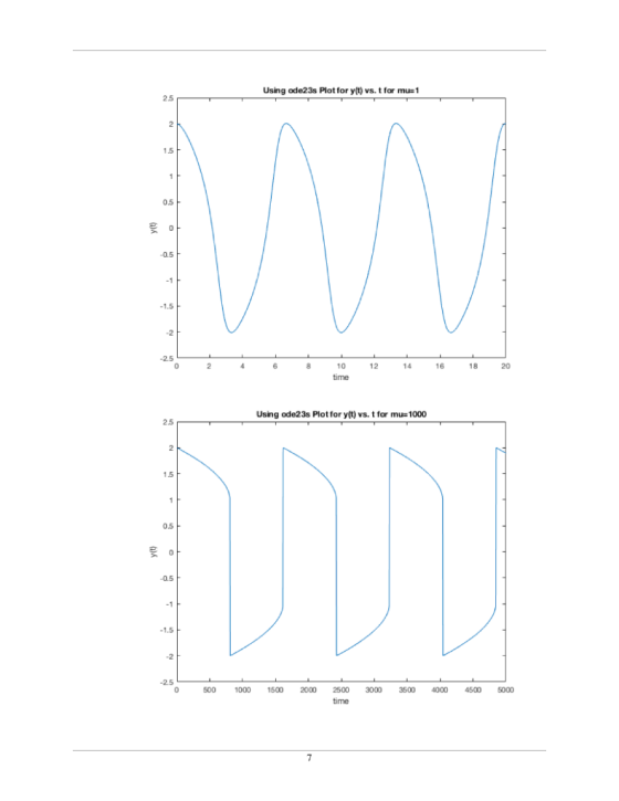
plot(t1,yy1(1,:))
title(sprintf('Using ode23 Plot for y(t) vs. t for mu=%d',mu1))
xlabel('time')
ylabel('y(t)')
ylim([-2.5 2.5])

figure(2)
plot(t2,yy2(1,:))
title(sprintf('Using ode23 Plot for y(t) vs. t for mu=%d',mu2))
xlabel('time')
ylabel('y(t)')
ylim([-2.5 2.5])

%Initial conditions for ode
    y0=[2;0];
    mu1=1; mu2=1000;
        %minimum and maximum time span
        tspan=[0 20];
        %Solution of ODEs using ode45 matlab function
        sol1= ode45(@(t,y) odefcn1(t,y,mu1), tspan, y0);
        %Equally splitting time into .02 sec interval for 0 to 50
        t1 = tspan(1):0.1:tspan(end);
        %yy is the corresponding x y v and z
        yy1 = deval(sol1,t1);
      
        y0=[2;0];
        tspan=[0 5000];
        %Solution of ODEs using ode45 matlab function
        sol2= ode45(@(t,y) odefcn1(t,y,mu2), tspan, y0);
        %Equally splitting time into .02 sec interval for 0 to 50
        t2 = linspace(tspan(1),tspan(end),1000);
        %yy is the corresponding x y v and z
        yy2 = deval(sol2,t2);
      
figure(3)
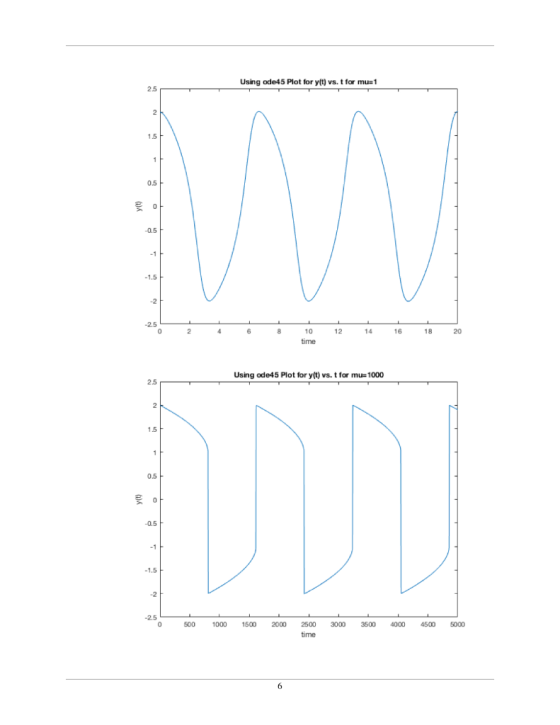
plot(t1,yy1(1,:))
title(sprintf('Using ode45 Plot for y(t) vs. t for mu=%d',mu1))
xlabel('time')
ylabel('y(t)')
ylim([-2.5 2.5])

figure(4)
plot(t2,yy2(1,:))
title(sprintf('Using ode45 Plot for y(t) vs. t for mu=%d',mu2))
xlabel('time')
ylabel('y(t)')
ylim([-2.5 2.5])

%Initial conditions for ode
    y0=[2;0];
    mu1=1; mu2=1000;
        %minimum and maximum time span
        tspan=[0 20];
        %Solution of ODEs using ode45 matlab function
        sol1= ode23s(@(t,y) odefcn1(t,y,mu1), tspan, y0);
        %Equally splitting time into .02 sec interval for 0 to 50
        t1 = tspan(1):0.1:tspan(end);
        %yy is the corresponding x y v and z
        yy1 = deval(sol1,t1);
      
        y0=[2;0];
        tspan=[0 5000];
        %Solution of ODEs using ode45 matlab function
        sol2= ode23s(@(t,y) odefcn1(t,y,mu2), tspan, y0);
        %Equally splitting time into .02 sec interval for 0 to 50
        t2 = linspace(tspan(1),tspan(end),1000);
        %yy is the corresponding x y v and z
        yy2 = deval(sol2,t2);
      
figure(5)
plot(t1,yy1(1,:))
title(sprintf('Using ode23s Plot for y(t) vs. t for mu=%d',mu1))
xlabel('time')
ylabel('y(t)')
ylim([-2.5 2.5])

figure(6)
plot(t2,yy2(1,:))
title(sprintf('Using ode23s Plot for y(t) vs. t for mu=%d',mu2))
xlabel('time')
ylabel('y(t)')
ylim([-2.5 2.5])

%Initial conditions for ode
    y0=[2;0];
    mu1=1; mu2=1000;
        %minimum and maximum time span
        tspan=[0 20];
        %Solution of ODEs using ode45 matlab function
        sol1= ode113(@(t,y) odefcn1(t,y,mu1), tspan, y0);
        %Equally splitting time into .02 sec interval for 0 to 50
        t1 = tspan(1):0.1:tspan(end);
        %yy is the corresponding x y v and z
        yy1 = deval(sol1,t1);
      
        y0=[2;0];
        tspan=[0 5000];
        %Solution of ODEs using ode45 matlab function
        sol2= ode113(@(t,y) odefcn1(t,y,mu2), tspan, y0);
        %Equally splitting time into .02 sec interval for 0 to 50
        t2 = linspace(tspan(1),tspan(end),1000);
        %yy is the corresponding x y v and z
        yy2 = deval(sol2,t2);
      
figure(7)
plot(t1,yy1(1,:))
title(sprintf('Using ode113 Plot for y(t) vs. t for mu=%d',mu1))
xlabel('time')
ylabel('y(t)')
ylim([-2.5 2.5])

figure(8)
plot(t2,yy2(1,:))
title(sprintf('Using ode113 Plot for y(t) vs. t for mu=%d',mu2))
xlabel('time')
ylabel('y(t)')
ylim([-2.5 2.5])

%Initial conditions for ode
    y0=[2;0];
    mu1=1; mu2=1000;
        %minimum and maximum time span
        tspan=[0 20];
        %Solution of ODEs using ode45 matlab function
        sol1= ode15s(@(t,y) odefcn1(t,y,mu1), tspan, y0);
        %Equally splitting time into .02 sec interval for 0 to 50
        t1 = tspan(1):0.1:tspan(end);
        %yy is the corresponding x y v and z
        yy1 = deval(sol1,t1);
      
        y0=[2;0];
        tspan=[0 5000];
        %Solution of ODEs using ode45 matlab function
        sol2= ode15s(@(t,y) odefcn1(t,y,mu2), tspan, y0);
        %Equally splitting time into .02 sec interval for 0 to 50
        t2 = linspace(tspan(1),tspan(end),1000);
        %yy is the corresponding x y v and z
        yy2 = deval(sol2,t2);
      
figure(9)
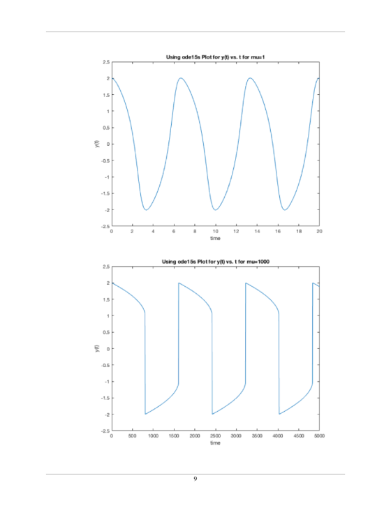
plot(t1,yy1(1,:))
title(sprintf('Using ode15s Plot for y(t) vs. t for mu=%d',mu1))
xlabel('time')
ylabel('y(t)')
ylim([-2.5 2.5])

figure(10)
plot(t2,yy2(1,:))
title(sprintf('Using ode15s Plot for y(t) vs. t for mu=%d',mu2))
xlabel('time')
ylabel('y(t)')
ylim([-2.5 2.5])

%Function for evaluating the ODE
function dydt = odefcn1(t,y,mu)

    eq1=y(2);
    eq2=-mu*((y(1)).^2-1).*y(2)-y(1);

    %Evaluate the ODE for our present problem
    dydt = [eq1;eq2];
  
end

%%%%%%%%%%%%%%%%% End of Code %%%%%%%%%%%%%