Question

Problem 3. Given the data points (xi, yi), with i0 1.2 2.3 3.5 4 yi 3.5 1.3 -0.7 0.5 2.7 find and plot (using MATLAB) the least-squares basis functions and the resulting least-squares fitting func- tions together with the given data points for the case of a) a linear monomial basis p (x) --{1x}T b) a quadratic monomial basis p(x)-1 x хут c) a trigonometric basis p (x)-{ l cos x sin x}T. Moreover, determine the coefficients a by the Moore-Penrose pseudoinverse V+. Lastly, calculate the least- squares error measure E2(a) for each case, and give a brief statement.

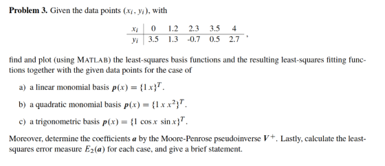
Given the data points (x_i , y_i), with

xi 0 1.2 2.3 3.5 4

yi 3.5 1.3 -0.7 0.5 2.7

find and plot (using MATLAB) the least-squares basis functions and the resulting least-squares fitting functions together with the given data points for the case of

a) a linear monomial basis p(x)= {1 x}^T .

b) a quadratic monomial basis p(x)= {1 x x²}^T .

c) a trigonometric basis p(x)= {1 cosx sinx}^T

Moreover, determine the coefficients a by the Moore-Penrose pseudoinverse V⁺. Lastly, calculate the leasts-squares error measure E₂(a) for each case, and give a brief statement.

Answer 1

MATLAB Code:

close all
clear
clc

x = [0 1.2 2.3 3.5 4]';
y = [3.5 1.3 -0.7 0.5 2.7]';
xx = min(x)-1:0.01:max(x)+1;
scatter(x,y), hold on

fprintf('Part (a)\n---------------------------------------------------\n')
V = [ones(size(x)) x];
a = pinv(V)*y; % Pseudo-Inverse
fprintf('Model: y = %f + %f*x\n', a)
plot(xx, a(1) + a(2)*xx)
error = norm(y - (a(1) + a(2)*x));
fprintf('Error: %f\n', error)

fprintf('\nPart (b)\n---------------------------------------------------\n')
V = [ones(size(x)) x x.^2];
a = pinv(V)*y;
fprintf('Model: y = %f + %f*x + %f*x^2\n', a)
plot(xx, a(1) + a(2)*xx + a(3)*xx.^2)
error = norm(y - (a(1) + a(2)*x + a(3)*x.^2));
fprintf('Error: %f\n', error)

fprintf('\nPart (c)\n---------------------------------------------------\n')
V = [ones(size(x)) cos(x) sin(x)];
a = pinv(V)*y;
fprintf('Model: y = %f + %f*cos(x) + %f*sin(x)\n', a)
plot(xx, a(1) + a(2)*cos(xx) + a(3)*sin(xx))
error = norm(y - (a(1) + a(2)*cos(x) + a(3)*sin(x)));
fprintf('Error: %f\n', error)

fprintf('\nHence, the trigonometric basis fits the data better.\n')

xlabel('x'), ylabel('y')
legend('Data Points', 'Part (a)', 'Part (b)', 'Part (c)')

Output:

Part (a)
---------------------------------------------------
Model: y = 2.186531 + -0.330241*x
Error: 3.183762

Part (b)
---------------------------------------------------
Model: y = 3.777155 + -3.653015*x + 0.817536*x^2
Error: 1.109697

Part (c)
---------------------------------------------------
Model: y = 1.990093 + 1.803397*cos(x) + -1.820891*sin(x)
Error: 0.826195

Hence, the trigonometric basis fits the data better.

Plot:

9 O Data Points Part (a) Part (b) Part (c) 6 4