Question

Collect a convenience sample (n = 100) of Oakland University undergraduate students on the following demographics information:
Gender (Female, Male)
Status (Full-Time, Part-Time)
County (Oakland, Other)
Major (SBA, Non-SBA).
You may get this data by asking any OU students that you know, in person, phone, email, text, etc. Then, compare this nonprobability sample you obtained with the known characteristics of the population (see the Sampling OU Students PowerPoint on Moodle) on each of the four demographic variables: Is this a representative sample? Calculate the Chi Square on each of the four demographic variables. Each Chi Square is a 2x2 table, so df = (columns-1)(rows-1) = 1. With df=1, the Chi Square critical value is 3.84 (see the Excel Tutorial Chi Square). Write a 1-page memo reporting your results, including your Chi Square calculations, so I can check your work.

1 Sample Size Gender Status County Major Other SBA OtherSBA Other SBA OtherSBA 5 M PT Other SBA OtherSBA Oakland SBA OtherSBA Other SBA OtherSBA Other SBA OtherSBA Oakland SBA OtherSBA Oakland Non-SBA OtherSBA Other SBA Oakland SBA Other SBA Oakland SBA Oakland SBA OtherSBA Other SBA Oakland SBA Other SBA Oakland SBA Oakland SBA OtherSBA Other SBA Oakland SBA Other SBA Oakland SBA Oakland SBA Oakland SBA Other SBA Oakland SBA Oakland SBA Oakland SBA Oakland SBA OtherSBA Oakland SBA Oakland SBA Other SBA Oakland SBA Oakland Non-SBA Oakland SBA Other SBA OtherSBA Other SBA OtherSBA 10 F 14 M 15 F 16 F 22 M 26 M 28 F 30 F 34 M 35 M 36 M 38 F 39 F 0 F 42 F 46 M 48 M 49 F

Answer 1

1) Chi-Square Goodness-of-Fit Test for Categorical Variable: gender

catagory	observed	test proportion	expected	contribution to chi sq
F	53	0.5	50	0.18
M	47	0.5	50	0.18

N	N*	DF	CHI-SQ	P-VALUE
100	0	1	0.36	0.549

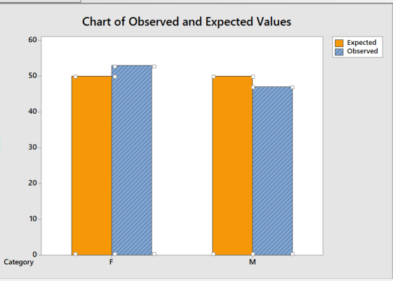
Explanation : As the graphs depict and As p-value=0.549>0.05 we accept the null hypothesis which says there is no significant difference between the population proportion and sample proportion of gender. This is also true as observed chi sq=0.36 < given chi sq=3.84, we accept the null hypothesis.

2) Chi-Square Goodness-of-Fit Test for Categorical Variable: status

catagory	observed	test proportion	expected	contribution to chi sq
FT	71	0.5	50	8.82
PT	29	0.5	50	8.82

N	N*	DF	CHI-SQ	P-VALUE
100	0	1	17.64	0

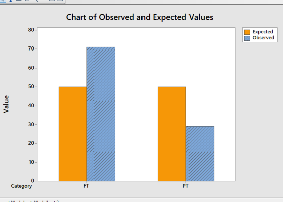
Explanation : As the graphs depict, The magnitude of the difference between the observed and expected values compared to its corresponding expected value is large and As p-value=0.000<0.05 we reject the null hypothesis which says there is no significant difference between the population proportion and sample proportion of status. This is also true as observed chi sq=17.64> given chi sq=3.84, we reject the null hypothesis.

3) Chi-Square Goodness-of-Fit Test for Categorical Variable: country

catagory	observed	test proportion	expected	contribution to chi sq
oakland	32	0.5	50	6.48
other	68	0.5	50	6.488

N	N*	DF	CHI-SQ	P-VALUE
100	0	1	12.96	0

Explanation : As the graphs depict, The magnitude of the difference between the observed and expected values compared to its corresponding expected value is large and As p-value=0.000<0.05 we reject the null hypothesis which says there is no significant difference between the population proportion and sample proportion of countries. This is also true as observed chi sq=12.96 > given chi sq=3.84, we reject the null hypothesis.

4) Chi-Square Goodness-of-Fit Test for Categorical Variable: major

catagory	observed	test proportion	expected	contribution to chi sq
Non SBA	7	0.5	50	36.98
SBA	93	0.5	50	36.98

N	N*	DF	CHI-SQ	P-VALUE
100	0	1	73.96	0

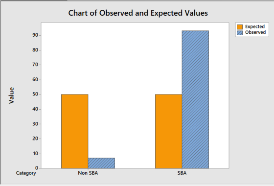
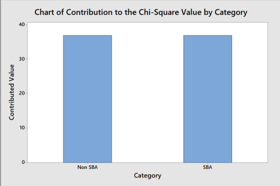
Explanation : As the graphs depict, The magnitude of the difference between the observed and expected values compared to its corresponding expected value is large and As p-value=0.000<0.05 we reject the null hypothesis which says there is no significant difference between the population proportion and sample proportion of major. This is also true as observed chi sq=73.96 > given chi sq=3.84, we reject the null hypothesis.