Question

(I did this homework in completion but professor was not happy with answers whatsoever, need additional answers and especially improvement to 1.b

help!! photos not attaching?

mean by severai steps. inis is a View Feedback homework and will need you to work, in one two View Feedback or various steps. Unfortunately, I cannot read your screen shot of what you did on excel. As I have said in numerous messages announcements etc, I cannot аcсept pictures. You need to write down on the homework format what you did on problem 1 on a table format, as a table is given to you. Write down the numbers as you see in the slides and practice problems. I've mentioned in several messages, announcements etc- what you see on the practice problems is what l expect to see in the homework. You can submit again. Hopefully you will have time to do this since we are so far away from the deadline. 8:05 AM 6/13/2019 Font Alignment Number Clipboard 30 H Column2 Column3 Column4 Columns Column6 Column7 Column& Column Column summary output 4regression stats 5 multiple r 0.905918994 5 r sq 0.820689224 7 adjr sq 0.77586153 B standard error 3.252589091 9 observation 6 11 ANOVA 2 df ms f sig f 3 regression 1 193.6826568 193.6827 18.30764 0.01286 4 residual 4 42.31734317 10.57934 15 total 5 236 16 17 coefficients standard error p value lower 95 % upper 95% lower 95.0 % upper 95.0 % t stat 18 intercept -8.487084871 7.247918529 -1.17097 0.306609 -28.6105 11.63636 -28.6105 11.63636 19 index 0.597785978 0.139710664 4.278743 0.01286 0.209887 0.985685 0.209887 0.985685 20 21 22 23 24 25 26 27 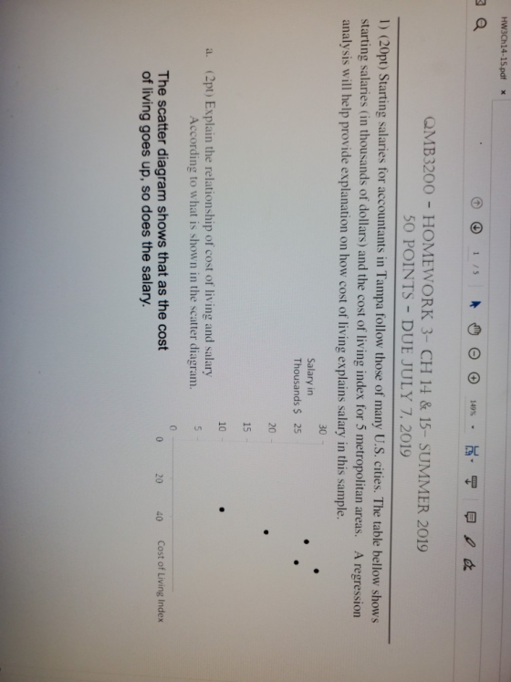HW3CH14-15.pdf 1/5 149% QMB3200 -HOMEWORK 3-CH 14 & 15-SUMMER 2019 50 POINTS - DUE JULY 7, 2019 1) (20pt) Starting salaries for accountants in Tampa follow those of many U.S. cities. The table bellow shows starting salaries (in thousands of dollars) and the cost of living index for 5 metropolitan areas. analysis will help provide explanation on how cost of living explains salary in this sample. A regression 30 Salary in Thousands $ 25 20 15 10 (2pt) Explain the relationship of cost of living and salary According to what is shown in the scatter diagram. a. The scatter diagram shows that as the cost of living goes up, so does the salary. 20 40 Cost of Living Index 149% b. (8pt)Use the least squares method (OLS) to develop an estimated regression equation for this problem (That is, calculate bo and bl) Metropolitan Salary (thousand S) area Index Oklahoma 46 19 City Tampa 35 10 Atlanta 50 27 Sacramento 65 29 Honolulu 59 25 Mean 51.0 22.0 view table that i submitted separately e MopuIM Help ools HW3Ch14-15.pdf 2 /5 + 149% (2pt) Write down the estimated regression equation. C. salary -8.48 +0.6 index interpretation for the slope. d. (3pt) Provide an slope is positive, +0.6 which means as the index/ order of the metropolital area increases, the starting salary increases too, by period of 0.6 of the order. 5 149% (5pt) Provide an interpretation for the intercept of the estimated regression equation. e. intercept is negative. The starting salary would be deducted by $8.48 thousand from what was predicted from the index of the city. HW3Ch14-15pdf Adobe Acrobat Reader DC le Edit View Window Help Home Tools HW3CH14-15.pdf 3 /5 149 % . 2) (30pt) The CEO of a well-known car reseller company wants to determine the factors having an influence on the resale value of a vehicle. The CEO knows that the resale value is an important factor considered by Search tools customers when buying a car. Assume you are performing a regression analysis using the data provided in the Export table below showing resale value, suggested price and type of vehicle (sport utility, small pickup). Adobe Export Convert PDF Files or Excel Onine Suggested Price ($) Resale (2pt) How would you include "Type of vehicle" in the regression analysis? Type of Vehicle Sport Utility a Vehicle Value (%) Select PDF File Chevrolet Blazer LS 19,495 5 HW3CH14-15.pd 20,495 57 Ford Explorer Sport GMC Yukon XL 1500 Sport Utility 26,789 67 Convert to You would make a binary replica of a variable for all of the factors of the variable, and use it in a linear reg model. Sport Utility Sport Utility Sport Utility Sport Utility Sport Utility Honda CR-V 18.965 65 Microsoft Word 30,186 62 Isuzu VehiCross Jeep Cherokee Limited Mercury Mountaineen Nissan Pathfinder XE Document Language English (U.S) Chang 25,745 29.895 59 Sport Utility Sport Utility Sport Utility Small Pickup 26.919 54 Toyota 4Runner Toyota RAV4 Cvevrolet S-10 Extended Cab Dodge Dakota Club Cab Sport Ford Ranger XLT Regular Cab Ford Ranger XLT Supercab GMC Sonoma Regular Cab Isuzu Hombre Spacecab 22.418 55 Convert 17.148 55 18.847 48 Create PDF Small Pickup Small Pickup 16.870 53 18.510 48 Edit PDF 55 Small Pickup Small Pickup 20.225 16.938 Comment 44 18.820 23.050 12.110 18.228 41 Small Pickup Combine Files 51 Small Pickup Small Pickup Mazda B4000 SE Cab Plus 51 Organize Page Nissan Frontier XE Regular 49 Small Pickup Small Pickup Small Pickup Toyota Tacoma Xtracab Redact 19.318 50 Toyota Tacoma XtracabV6 Toyota Tacoma XtracabV8 12.000 70 Send, sign, and trac POFS Orrnlo wtn Tools HW3Ch14-15.pdf 3/5 149% SEPT 1: A REGRESSION IS ESTIMATED USING ONLY SUGGESTEDPRICE (2pt) Comment on the goodness of fit of the MODEL. a. Model Summary Adjusted R Square 166 Std. Error of the Estimate 6.271 The value of R^2 is 0.193, which is near zero. The 19.3 variability of resale value can be explained by the suggested price. The model is not good. Model R Square .193 440a a. Predictors: (Constant), Suggested Price b. Dependent Variable: Resalevalue HWCh14-15pdf- Adobe Acrobat Reader DC File Edit View Window Help Home Tools HW3Ch14-15.pdf x 4 /5 125% . b. (2pt) Explain whether normality assumptions hold (or not) for this model Search tools Yes, the normality assumptions hold becasue the graph does Export not have a pattern. Adobe Export Convert PDF Files It is randomly distributed or Excel Online Select PDF File And, the errors are near zero. HW3CH14-15 pd Convert to Microsoft Word t Document Language Regression Standardized Predicted Value English (US) Chang Convert Create PDF a. (2pt) Report the statistical significance of the MODEL Edit PDF ANOVA Sum of Comment Mean Souare 273 373 df 0.013 is the statistical significance, which means Si 0134 Model Sc Regression 273.373 5 952 the model itself is Combine Files Residual 1140.369 15 39 323 significant. The observed value of F statistic is 6.952 The p-value resulting P[F1,15 6.952] = 0.011868238. The model does not represent the effect at 1% level of significance, but at 5% we can say the model does have an effect. Total 1413 742 Organize Page 16 a Predictors (Constant), Su b Dependent Vatiable Resalevalue from this will be dPrice Redact level Stt Free Tia re Proben witn RS paying/Clitnt: Home Tools HW3Ch14-15.pdf x 4 /5 125% SEPT 2: Assume the variable SPORT is 1 if type of vehicle is sport utility, and = 0 otherwise. A regression is estimated using Suggested-price and SPORT (2pt) Comment on the goodness of fit for the model in STEP 2. a Model Summary Std Error of the Estimate Model R Square Adjusted R Square 631 The r-square value is 0.631. 63.1 % means that the model explains the variability of the resale value around its mean. 63.1% the 1 794 588 4 298 a Predictors: (Constant), SuggestedPrice, Sport Dependent Variable: ResaleValue data fit in the model. b. (1pt) Write down the estimated regression equation for this model. Coefficients resale value = 42.554 +0.000 (suggested price)+ 7.917 (sport) On Standardized Unstandardized Coefficients Coefficients Sia Model B Std. Error Beta (Constant) 42 554 3.562 11.947 000 080 270 567 1 89 000 2.163 SuggestedPrice 000 001 7917 Sport witn re:proden crobat Reader DC Help HW3Ch14-15.pdf x 5/5 100% (6pt) Report the statistical significance of the coefficients. c. rejection rule (p value method): if p-value a(0.05), therefore it Ish't staustically significant. sport p-value is 0.001 which

Answer 1

1.

a) From the scatter plot, we get to know that there is positive correlation between the cost of living index and salary i.e. salary can be decided using cost of living index.

b)

Area	Index (x)	Salary(y)	X - Mx	Y - My	(X - Mx)2	(X - Mx)(Y - My)
Oklahoma city	46	19	-5	-3	25	15
Tampa	35	10	-16	-12	256.00	192
atlanta	50	27	-1	5	1	-5
sacramanto	65	29	14	7	196	98
honolulu	59	25	8	3	64	24
sum					542	324

Sum of X = 255

Sum of Y = 110

Mean X = 51

Mean Y = 22

Sum of squares (SSX) = 542

Sum of products (SP) = 324

Regression Equation = ŷ = bX + a

b = SP/SSX = 324/542 = 0.59779

a = MY - bMX = 22 - (0.6*51) = -8.48708

ŷ = 0.59779X - 8.48708

d) The slope is positive here. The coefficient indicates that for every unit change in cost of living index you can expect salary to increase by an average of 0.6 thousand dollar

e)  From the regression equation, we see that the intercept value is -8.48. If the value of cost of living index is zero, the regression equation predicts that salary is -8.48 thousand dollar!

All the answers are just fine!