Apply Euler-trapezoidal predictor-corrector method to the IVP in problem 1 to approximate y(2), by choosing two values of h, for which the iteration converges. (Don't really need to show work or do by hand, MATLAB code will work just as well).

Homework Answers

Add Answer to:
Apply Euler-trapezoidal predictor-corrector method to the IVP in problem 1 to approximate y(2), by choosing two...
For the IVP: Apply Euler-trapezoidal predictor-corrector method to the IVP to approximate y(2), by choosing two...
 For the IVP:
Apply Euler-trapezoidal predictor-corrector method to the IVP to
approximate y(2), by choosing two values of h, for which the
iteration converges. (Note: True Solution: y(t) = et − t
− 1). Present your results in tabular form. Your tabulated results
must contain the exact value, approximate value by the
Euler-trapezoidal predictor-corrector method at t0 = 0,
t1 = 0.5, t2 = 1, t3 = 1.5,
t4 = 2, t5 = 2.5, t6 = 3,
t7 = 3.5...
For the IVP:
Apply Euler-trapezoidal predictor-corrector method to the IVP to
approximate y(2), by choosing two values of h, for which the
iteration converges. (Note: True Solution: y(t) = et − t
− 1). Present your results in tabular form. Your tabulated results
must contain the exact value, approximate value by the
Euler-trapezoidal predictor-corrector method at t0 = 0,
t1 = 0.5, t2 = 1, t3 = 1.5,
t4 = 2, t5 = 2.5, t6 = 3,
t7 = 3.5...
Problem 1 Use Euler's method with step size h = 0.5 to approximate the solution of the IVP. 2 dy ...
 Problem 1 Use Euler's method with step size h = 0.5 to approximate the solution of the IVP. 2 dy ev dt t 1-t-2, y(1) = 0. Problem 2 Consider the IVP: dy dt (a) Use Euler's method with step size h0.25 to approximate y(0.5) b) Find the exact solution of the IV P c) Find the maximum error in approximating y(0.5) by y2 (d) Calculate the actual absolute error in approximating y(0.5) by /2.
Problem 1 Use Euler's method...
Problem 1 Use Euler's method with step size h = 0.5 to approximate the solution of the IVP. 2 dy ev dt t 1-t-2, y(1) = 0. Problem 2 Consider the IVP: dy dt (a) Use Euler's method with step size h0.25 to approximate y(0.5) b) Find the exact solution of the IV P c) Find the maximum error in approximating y(0.5) by y2 (d) Calculate the actual absolute error in approximating y(0.5) by /2.
Problem 1 Use Euler's method...
Solve using Matlab Use the forward Euler method, Vi+,-Vi+(4+1-tinti ,Vi) for i= 0,1,2, , taking yo y(to) to be the initial condition, to approximate the solution at t-2 of the IVP y'=y-t2 + 1, 0-...
 Solve using Matlab
Use the forward Euler method, Vi+,-Vi+(4+1-tinti ,Vi) for i= 0,1,2, , taking yo y(to) to be the initial condition, to approximate the solution at t-2 of the IVP y'=y-t2 + 1, 0-t-2, y(0) = 0.5. Use N = 2k, k = 1, 2, , 20 equispaced time steps (so to = 0 and tN-1 = 2). Make a convergence plot, computing the error by comparing with the exact solution, y: t1)2 -exp(t)/2, and plotting the error as...
Solve using Matlab
Use the forward Euler method, Vi+,-Vi+(4+1-tinti ,Vi) for i= 0,1,2, , taking yo y(to) to be the initial condition, to approximate the solution at t-2 of the IVP y'=y-t2 + 1, 0-t-2, y(0) = 0.5. Use N = 2k, k = 1, 2, , 20 equispaced time steps (so to = 0 and tN-1 = 2). Make a convergence plot, computing the error by comparing with the exact solution, y: t1)2 -exp(t)/2, and plotting the error as...
[7] 1. Consider the initial value problem (IVP) y′(t) = −y(t), y(0) = 1 The solution to this IVP ...
[7] 1. Consider the initial value problem (IVP) y′(t) = −y(t), y(0) = 1 The solution to this IVP is y(t) = e−t [1] i) Implement Euler’s method and generate an approximate solution of this IVP over the interval [0,2], using stepsize h = 0.1. (The Google sheet posted on LEARN is set up to carry out precisely this task.) Report the resulting approximation of the value y(2). [1] ii) Repeat part (ii), but use stepsize h = 0.05. Describe...
1. Consider the IVP y = 1 - 100(y-t), y(0) = 0.5. (a) Find the exact...
 1. Consider the IVP y = 1 - 100(y-t), y(0) = 0.5. (a) Find the exact solution. (b) Use the Forward Euler, Heun, and Backward Euler methods to find approximate solu- tions ont € 0, 0.5], using h = 0.25. Plot all four solutions (exact and three approxima- tions) on the same graph. (c) Maple's approximation is plotted, along with the direction field, in Figure 1. Use it, and the exact solution, to explain the behaviours observed in your numerical...
MATLAB help please!!!!! 1. Use the forward Euler method Vi+,-Vi + (ti+1-tinti , yi) for i=0.1, 2, , taking yo-y(to) to be the initial condition, to approximate the solution at 2 of the IVP y'=y-t...
 MATLAB help please!!!!!
1. Use the forward Euler method Vi+,-Vi + (ti+1-tinti , yi) for i=0.1, 2, , taking yo-y(to) to be the initial condition, to approximate the solution at 2 of the IVP y'=y-t2 + 1, 0 2, y(0) = 0.5. t Use N 2k, k2,...,20 equispaced timesteps so to 0 and t-1 2) Make a convergence plot computing the error by comparing with the exact solution, y: t (t+1)2 exp(t)/2, and plotting the error as a function of...
MATLAB help please!!!!!
1. Use the forward Euler method Vi+,-Vi + (ti+1-tinti , yi) for i=0.1, 2, , taking yo-y(to) to be the initial condition, to approximate the solution at 2 of the IVP y'=y-t2 + 1, 0 2, y(0) = 0.5. t Use N 2k, k2,...,20 equispaced timesteps so to 0 and t-1 2) Make a convergence plot computing the error by comparing with the exact solution, y: t (t+1)2 exp(t)/2, and plotting the error as a function of...
Given the ODE and initial condition 3. y(0) = 1 dt=yi-y Use the explicit predictor-corrector (Heun's)...
 Given the ODE and initial condition 3. y(0) = 1 dt=yi-y Use the explicit predictor-corrector (Heun's) method to manually (i.e. on paper, by hand use Matlab as a calculator, however) integrate this from t -0 to t 1.5 using h 0.5. Describe technique in words and/or equations and fill out the table below with this solution att -[0.0,0.s -you may you i Ss Step 1 Step 2 Step 3 y'(0.0) = y'(0.5) = (0.5)
. Consider the IVP y'= 1 + y?, y(0) = 0 a. Solve the IVP analytically...
 . Consider the IVP y'= 1 + y?, y(0) = 0 a. Solve the IVP analytically b. Using step size 0.1, approximate y(0.5) using Euler's Method c. Using step size 0.1, approximate y(0.5) using Euler's Improved Method d. Find the error between the analytic solution and both methods at each step
Adams Fourth-Order Predictor-Corrector Python ONLY!! Please translate this pseudocode into Python code, thanks!! Adams Fourth-Order Predictor-Corrector...
 Adams Fourth-Order Predictor-Corrector Python ONLY!!
Please translate this pseudocode into Python code, thanks!!
Adams Fourth-Order Predictor-Corrector To approximate the solution of the initial-value problem y' = f(t, y), ast<b, y(a) = a, at (N + 1) equally spaced numbers in the interval [a, b]: INPUT endpoints a, b; integer N; initial condition a. OUTPUT approximation w to y at the (N + 1) values of t. Step 1 Set h = (b − a)/N; to = a; Wo = a;...
Adams Fourth-Order Predictor-Corrector Python ONLY!!
Please translate this pseudocode into Python code, thanks!!
Adams Fourth-Order Predictor-Corrector To approximate the solution of the initial-value problem y' = f(t, y), ast<b, y(a) = a, at (N + 1) equally spaced numbers in the interval [a, b]: INPUT endpoints a, b; integer N; initial condition a. OUTPUT approximation w to y at the (N + 1) values of t. Step 1 Set h = (b − a)/N; to = a; Wo = a;...
Numerical Methods Consider the following IVP dy=0.01(70-y)(50-y), with y(0)-0 (a) [10 marks Use the Runge-Kutta method of order four to obtain an approximate solution to the ODE at the points t-0.5 an...
 Numerical Methods
Consider the following IVP dy=0.01(70-y)(50-y), with y(0)-0 (a) [10 marks Use the Runge-Kutta method of order four to obtain an approximate solution to the ODE at the points t-0.5 and t1 with a step sizeh 0.5. b) [8 marks Find the exact solution analytically. (c) 7 marks] Use MATLAB to plot the graph of the true and approximate solutions in one figure over the interval [.201. Display graphically the true errors after each steps of calculations.
Consider the...
Numerical Methods
Consider the following IVP dy=0.01(70-y)(50-y), with y(0)-0 (a) [10 marks Use the Runge-Kutta method of order four to obtain an approximate solution to the ODE at the points t-0.5 and t1 with a step sizeh 0.5. b) [8 marks Find the exact solution analytically. (c) 7 marks] Use MATLAB to plot the graph of the true and approximate solutions in one figure over the interval [.201. Display graphically the true errors after each steps of calculations.
Consider the...
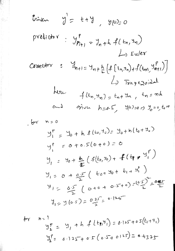
 For the IVP:
Apply Euler-trapezoidal predictor-corrector method to the IVP to
approximate y(2), by choosing two values of h, for which the
iteration converges. (Note: True Solution: y(t) = et − t
− 1). Present your results in tabular form. Your tabulated results
must contain the exact value, approximate value by the
Euler-trapezoidal predictor-corrector method at t0 = 0,
t1 = 0.5, t2 = 1, t3 = 1.5,
t4 = 2, t5 = 2.5, t6 = 3,
t7 = 3.5...
For the IVP:
Apply Euler-trapezoidal predictor-corrector method to the IVP to
approximate y(2), by choosing two values of h, for which the
iteration converges. (Note: True Solution: y(t) = et − t
− 1). Present your results in tabular form. Your tabulated results
must contain the exact value, approximate value by the
Euler-trapezoidal predictor-corrector method at t0 = 0,
t1 = 0.5, t2 = 1, t3 = 1.5,
t4 = 2, t5 = 2.5, t6 = 3,
t7 = 3.5...
 Problem 1 Use Euler's method with step size h = 0.5 to approximate the solution of the IVP. 2 dy ev dt t 1-t-2, y(1) = 0. Problem 2 Consider the IVP: dy dt (a) Use Euler's method with step size h0.25 to approximate y(0.5) b) Find the exact solution of the IV P c) Find the maximum error in approximating y(0.5) by y2 (d) Calculate the actual absolute error in approximating y(0.5) by /2.
Problem 1 Use Euler's method...
Problem 1 Use Euler's method with step size h = 0.5 to approximate the solution of the IVP. 2 dy ev dt t 1-t-2, y(1) = 0. Problem 2 Consider the IVP: dy dt (a) Use Euler's method with step size h0.25 to approximate y(0.5) b) Find the exact solution of the IV P c) Find the maximum error in approximating y(0.5) by y2 (d) Calculate the actual absolute error in approximating y(0.5) by /2.
Problem 1 Use Euler's method...
 Solve using Matlab
Use the forward Euler method, Vi+,-Vi+(4+1-tinti ,Vi) for i= 0,1,2, , taking yo y(to) to be the initial condition, to approximate the solution at t-2 of the IVP y'=y-t2 + 1, 0-t-2, y(0) = 0.5. Use N = 2k, k = 1, 2, , 20 equispaced time steps (so to = 0 and tN-1 = 2). Make a convergence plot, computing the error by comparing with the exact solution, y: t1)2 -exp(t)/2, and plotting the error as...
Solve using Matlab
Use the forward Euler method, Vi+,-Vi+(4+1-tinti ,Vi) for i= 0,1,2, , taking yo y(to) to be the initial condition, to approximate the solution at t-2 of the IVP y'=y-t2 + 1, 0-t-2, y(0) = 0.5. Use N = 2k, k = 1, 2, , 20 equispaced time steps (so to = 0 and tN-1 = 2). Make a convergence plot, computing the error by comparing with the exact solution, y: t1)2 -exp(t)/2, and plotting the error as...
 1. Consider the IVP y = 1 - 100(y-t), y(0) = 0.5. (a) Find the exact solution. (b) Use the Forward Euler, Heun, and Backward Euler methods to find approximate solu- tions ont € 0, 0.5], using h = 0.25. Plot all four solutions (exact and three approxima- tions) on the same graph. (c) Maple's approximation is plotted, along with the direction field, in Figure 1. Use it, and the exact solution, to explain the behaviours observed in your numerical...
 MATLAB help please!!!!!
1. Use the forward Euler method Vi+,-Vi + (ti+1-tinti , yi) for i=0.1, 2, , taking yo-y(to) to be the initial condition, to approximate the solution at 2 of the IVP y'=y-t2 + 1, 0 2, y(0) = 0.5. t Use N 2k, k2,...,20 equispaced timesteps so to 0 and t-1 2) Make a convergence plot computing the error by comparing with the exact solution, y: t (t+1)2 exp(t)/2, and plotting the error as a function of...
MATLAB help please!!!!!
1. Use the forward Euler method Vi+,-Vi + (ti+1-tinti , yi) for i=0.1, 2, , taking yo-y(to) to be the initial condition, to approximate the solution at 2 of the IVP y'=y-t2 + 1, 0 2, y(0) = 0.5. t Use N 2k, k2,...,20 equispaced timesteps so to 0 and t-1 2) Make a convergence plot computing the error by comparing with the exact solution, y: t (t+1)2 exp(t)/2, and plotting the error as a function of...
 Given the ODE and initial condition 3. y(0) = 1 dt=yi-y Use the explicit predictor-corrector (Heun's) method to manually (i.e. on paper, by hand use Matlab as a calculator, however) integrate this from t -0 to t 1.5 using h 0.5. Describe technique in words and/or equations and fill out the table below with this solution att -[0.0,0.s -you may you i Ss Step 1 Step 2 Step 3 y'(0.0) = y'(0.5) = (0.5)
 . Consider the IVP y'= 1 + y?, y(0) = 0 a. Solve the IVP analytically b. Using step size 0.1, approximate y(0.5) using Euler's Method c. Using step size 0.1, approximate y(0.5) using Euler's Improved Method d. Find the error between the analytic solution and both methods at each step
 Adams Fourth-Order Predictor-Corrector Python ONLY!!
Please translate this pseudocode into Python code, thanks!!
Adams Fourth-Order Predictor-Corrector To approximate the solution of the initial-value problem y' = f(t, y), ast<b, y(a) = a, at (N + 1) equally spaced numbers in the interval [a, b]: INPUT endpoints a, b; integer N; initial condition a. OUTPUT approximation w to y at the (N + 1) values of t. Step 1 Set h = (b − a)/N; to = a; Wo = a;...
Adams Fourth-Order Predictor-Corrector Python ONLY!!
Please translate this pseudocode into Python code, thanks!!
Adams Fourth-Order Predictor-Corrector To approximate the solution of the initial-value problem y' = f(t, y), ast<b, y(a) = a, at (N + 1) equally spaced numbers in the interval [a, b]: INPUT endpoints a, b; integer N; initial condition a. OUTPUT approximation w to y at the (N + 1) values of t. Step 1 Set h = (b − a)/N; to = a; Wo = a;...
 Numerical Methods
Consider the following IVP dy=0.01(70-y)(50-y), with y(0)-0 (a) [10 marks Use the Runge-Kutta method of order four to obtain an approximate solution to the ODE at the points t-0.5 and t1 with a step sizeh 0.5. b) [8 marks Find the exact solution analytically. (c) 7 marks] Use MATLAB to plot the graph of the true and approximate solutions in one figure over the interval [.201. Display graphically the true errors after each steps of calculations.
Consider the...
Numerical Methods
Consider the following IVP dy=0.01(70-y)(50-y), with y(0)-0 (a) [10 marks Use the Runge-Kutta method of order four to obtain an approximate solution to the ODE at the points t-0.5 and t1 with a step sizeh 0.5. b) [8 marks Find the exact solution analytically. (c) 7 marks] Use MATLAB to plot the graph of the true and approximate solutions in one figure over the interval [.201. Display graphically the true errors after each steps of calculations.
Consider the...
Most questions answered within 3 hours.
-
Find the mixed-strategy equilibrium to the Battle of the sexes
game in Figure 5.1 below
Hockey...
asked 3 minutes ago -
At 1 bar, how much energy is required to heat 61.0 g of H2O(s)
at −12.0...
asked 1 minute ago -
Use the following information to answer the next three
questions.
QUESTION 5
As of today, the...
asked 8 minutes ago -
Using the specific identification method: Date Units purchased
Cost per unit Ending inventory March 1 15...
asked 11 minutes ago -
PLEASE HELP, NO ONE IS ANSWERING MY QUESTION AND IT IS SUE TODAY
WORTH 20% OF...
asked 25 minutes ago -
α = 0.0007889 T, I = 2.9 A
Other Magnetic Fields: First, based on your
value...
asked 25 minutes ago -
This assignment is a continuation of the 2nd one. You as a HR
Manager, select an...
asked 27 minutes ago -
Hastings Entertainment has a beta of 0.64. If the market return
is expected to be 13.80...
asked 39 minutes ago -
9. Depository institutions are always:
a. illiquid
b. profitable
c. insolvent
d. all of the above...
asked 47 minutes ago -
Use AstroTurf Company's income statement below to answer the
following two questions. Answer these questions with...
asked 47 minutes ago -
How is a firm's task
environment different from its general environment? Provide
examples of both types...
asked 45 minutes ago -
What is one reason Innovators can adopt innovations so
early?
Group of answer choices
they are...
asked 47 minutes ago