![4. Now we return to the red and green dice from Homework 1. Use the lines below to simulate the random variables from Doughertys Chapter 1 problems, and then use R to estimate the answers to each of the problems below. ## Generating the Random Variables for Pages 13 and 14 red - sample (c(1:6),repl-T, size-10000) green = sample(c(1:6),repl-T,size-10000) sum = red-green max - ifelse (red > green, red, green) diff abs(red-green) table (sum) ## sum ## 2 3 4 5 6 7 8 9 10 11 12 ## 281 605 806 1075 1333 1679 1401 1123 841 576 280 mean (sum) ## [1] 7.0148 mean (sum 2) ## [1] 55.1342 var (sum) ## [1] 5.927374 sd (sum) ## [1] 2.43462 sum( (sum-mean (sum)) 2/9999 ## [1] 5.927374 mean (sum 2)-mean (sum)2 ## [1] 5.926781 Why doesnt the last expression equal the other variances? (Because mean divides by n and not n - 1 hist (sum)](http://img.homeworklib.com/questions/bd3e66e0-5cf8-11ea-8880-7b881b6f3e0d.png?x-oss-process=image/resize,w_560)
Need help with the codings in R Markdown (in R Studio)
Homework Answers
Sol: Since sample mean and sample variance is unbiased estimator of population mean and population variance respectively.
and
Where,
is a sample
mean and
is a population
mean.
is sample variance.
is population variance.
Therefore, R-code result gives approximately same value of sample variance (dividing by n-1) and population variance (dividing by n)
> red=sample(c(1:6),repl=T,size=10000)
> green=sample(c(1:6),repl=T,size=10000)
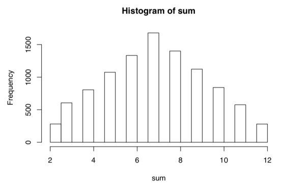
> sum=red+green
> max=ifelse(red>green, red, green)
> diff=abs(red-green)
> table(sum)
sum
2 3
4 5 6
7 8 9
10 11 12
270 555 850 1132 1380 1649 1372 1084 848 591 269
> mean(sum)
[1] 7.0029
> mean(sum^2)
[1] 54.9115
> var(sum)
[1] 5.871479
> sd(sum)
[1] 2.423113
> sum((sum-mean(sum))^2)/9999 # This case provides sample
variance.
[1] 5.871479
> mean(sum^2)-mean(sum)^2 # This case provides
population variance.
[1] 5.870892
> hist(sum)
Add Answer to:
Need help with the codings in R Markdown (in R Studio)
Preview of Homework 1 R.1...
PLEASE HELP WITH THE FOLLOWING R CODE! I NEED HELP WITH PART C AND D, provided...
 PLEASE HELP WITH THE FOLLOWING R CODE!
I NEED HELP WITH PART C AND D,
provided is part a and b!!!!
a)
chiNum <- c()
for (i in 1:1000)
{
g1 <- rnorm(20,10,4)
g2 <- rnorm(20,10,4)
g3 <- rnorm(20,10,4)
g4 <- rnorm(20,10,4)
g5 <- rnorm(20,10,4)
g6 <- rnorm(20,10,4)
mse <- (var(g1)+var(g2)+var(g3)+var(g4)+var(g5)+var(g6))/6
M <-
(mean(g1)+mean(g2)+mean(g3)+mean(g4)+mean(g5)+mean(g6))/6
msb <-
((((mean(g1)-M)^2)+((mean(g2)-M)^2)+((mean(g3)-M)^2)+((mean(g4)-M)^2)+((mean(g5)-M)^2)+((mean(g6)-M)^2))/5)*20
chiNum[i] <- msb/mse
}
# plot a histogram of F statistics
h <- hist(chiNum,plot=FALSE)
ylim <- (range(0, 0.8))
x <- seq(0,6,0.01)
hist(chiNum,freq=FALSE, ylim=ylim)...
PLEASE HELP WITH THE FOLLOWING R CODE!
I NEED HELP WITH PART C AND D,
provided is part a and b!!!!
a)
chiNum <- c()
for (i in 1:1000)
{
g1 <- rnorm(20,10,4)
g2 <- rnorm(20,10,4)
g3 <- rnorm(20,10,4)
g4 <- rnorm(20,10,4)
g5 <- rnorm(20,10,4)
g6 <- rnorm(20,10,4)
mse <- (var(g1)+var(g2)+var(g3)+var(g4)+var(g5)+var(g6))/6
M <-
(mean(g1)+mean(g2)+mean(g3)+mean(g4)+mean(g5)+mean(g6))/6
msb <-
((((mean(g1)-M)^2)+((mean(g2)-M)^2)+((mean(g3)-M)^2)+((mean(g4)-M)^2)+((mean(g5)-M)^2)+((mean(g6)-M)^2))/5)*20
chiNum[i] <- msb/mse
}
# plot a histogram of F statistics
h <- hist(chiNum,plot=FALSE)
ylim <- (range(0, 0.8))
x <- seq(0,6,0.01)
hist(chiNum,freq=FALSE, ylim=ylim)...
Need help for the coding using the R Markdown in R Studio for question2 and question2....
 Need help for the coding using the R Markdown in R Studio for
question2 and question2. Please provide a detailed solution with an
original R code, outputs and a clear statement of the final
answer.
First, verify by typing out the terms in the appropriate formulas for the t-statistic and the confidence limits that you and R agree about how these should be calculated. For instance, your R code should be structured the way the Excel commands for confidence limits...
Need help for the coding using the R Markdown in R Studio for
question2 and question2. Please provide a detailed solution with an
original R code, outputs and a clear statement of the final
answer.
First, verify by typing out the terms in the appropriate formulas for the t-statistic and the confidence limits that you and R agree about how these should be calculated. For instance, your R code should be structured the way the Excel commands for confidence limits...
R studio #Exercise : Calculate the following probabilities : #1. Probability that a normal random variable...
R studio #Exercise : Calculate the following probabilities : #1. Probability that a normal random variable with mean 22 and variance 25 #(i)lies between 16.2 and 27.5 #(ii) is greater than 29 #(iii) is less than 17 #(iv)is less than 15 or greater than 25 #2.Probability that in 60 tosses of a fair coin the head comes up #(i) 20,25 or 30 times #(ii) less than 20 times #(iii) between 20 and 30 times #3.A random variable X has Poisson...
Consider the number of days absent from a random sample of six students during a semester:...
Consider the number of days absent from a random sample of six students during a semester: A= {2, 3, 2, 4, 2, 5} Compute the arithmetic mean, geometric mean, median, and mode by hand and verify the results using R Arithmetic Mean: X=i=1nXin=2+3+2+4+2+56=3 mean(data2$absent) [1] 3 Geometic Mean: GMx=Πi=1nX11n=2∙3∙2∙4∙2∙516=2.79816 >gmean <- prod(data2$absent)^(1/length(data2$absent)) > gmean [1] 2.798166 Median: X=12n+1th, Xi2,2,2,3,4,5, n=6=126+1th ranked value=3.5, value=2.5 days absent >median(data2$absent) [1] 2.5 Mode: Most frequent value=2 > mode <- names(table(data2$absent)) [table(data2$absent)==max(table(data2$absent))] > mode [1]...
For expert using R , I solve it but i need to figure out what I...
 For expert using R , I solve it but i need to figure out what
I got is correct or wrong. Thank you
# Simple Linear Regression and Polynomial Regression
# HW 2
#
# Read data from csv file
data <-
read.csv("C:\data\SweetPotatoFirmness.csv",header=TRUE,
sep=",")
head(data)
str(data)
# scatterplot of independent and dependent variables
plot(data$pectin,data$firmness,xlab="Pectin,
%",ylab="Firmness")
par(mfrow = c(2, 2)) # Split the plotting panel into a 2 x 2
grid
model <- lm(firmness ~ pectin , data=data)
summary(model)
anova(model)
plot(model)...
For expert using R , I solve it but i need to figure out what
I got is correct or wrong. Thank you
# Simple Linear Regression and Polynomial Regression
# HW 2
#
# Read data from csv file
data <-
read.csv("C:\data\SweetPotatoFirmness.csv",header=TRUE,
sep=",")
head(data)
str(data)
# scatterplot of independent and dependent variables
plot(data$pectin,data$firmness,xlab="Pectin,
%",ylab="Firmness")
par(mfrow = c(2, 2)) # Split the plotting panel into a 2 x 2
grid
model <- lm(firmness ~ pectin , data=data)
summary(model)
anova(model)
plot(model)...
 PLEASE HELP WITH THE FOLLOWING R CODE!
I NEED HELP WITH PART C AND D,
provided is part a and b!!!!
a)
chiNum <- c()
for (i in 1:1000)
{
g1 <- rnorm(20,10,4)
g2 <- rnorm(20,10,4)
g3 <- rnorm(20,10,4)
g4 <- rnorm(20,10,4)
g5 <- rnorm(20,10,4)
g6 <- rnorm(20,10,4)
mse <- (var(g1)+var(g2)+var(g3)+var(g4)+var(g5)+var(g6))/6
M <-
(mean(g1)+mean(g2)+mean(g3)+mean(g4)+mean(g5)+mean(g6))/6
msb <-
((((mean(g1)-M)^2)+((mean(g2)-M)^2)+((mean(g3)-M)^2)+((mean(g4)-M)^2)+((mean(g5)-M)^2)+((mean(g6)-M)^2))/5)*20
chiNum[i] <- msb/mse
}
# plot a histogram of F statistics
h <- hist(chiNum,plot=FALSE)
ylim <- (range(0, 0.8))
x <- seq(0,6,0.01)
hist(chiNum,freq=FALSE, ylim=ylim)...
PLEASE HELP WITH THE FOLLOWING R CODE!
I NEED HELP WITH PART C AND D,
provided is part a and b!!!!
a)
chiNum <- c()
for (i in 1:1000)
{
g1 <- rnorm(20,10,4)
g2 <- rnorm(20,10,4)
g3 <- rnorm(20,10,4)
g4 <- rnorm(20,10,4)
g5 <- rnorm(20,10,4)
g6 <- rnorm(20,10,4)
mse <- (var(g1)+var(g2)+var(g3)+var(g4)+var(g5)+var(g6))/6
M <-
(mean(g1)+mean(g2)+mean(g3)+mean(g4)+mean(g5)+mean(g6))/6
msb <-
((((mean(g1)-M)^2)+((mean(g2)-M)^2)+((mean(g3)-M)^2)+((mean(g4)-M)^2)+((mean(g5)-M)^2)+((mean(g6)-M)^2))/5)*20
chiNum[i] <- msb/mse
}
# plot a histogram of F statistics
h <- hist(chiNum,plot=FALSE)
ylim <- (range(0, 0.8))
x <- seq(0,6,0.01)
hist(chiNum,freq=FALSE, ylim=ylim)...
 Need help for the coding using the R Markdown in R Studio for
question2 and question2. Please provide a detailed solution with an
original R code, outputs and a clear statement of the final
answer.
First, verify by typing out the terms in the appropriate formulas for the t-statistic and the confidence limits that you and R agree about how these should be calculated. For instance, your R code should be structured the way the Excel commands for confidence limits...
Need help for the coding using the R Markdown in R Studio for
question2 and question2. Please provide a detailed solution with an
original R code, outputs and a clear statement of the final
answer.
First, verify by typing out the terms in the appropriate formulas for the t-statistic and the confidence limits that you and R agree about how these should be calculated. For instance, your R code should be structured the way the Excel commands for confidence limits...
 For expert using R , I solve it but i need to figure out what
I got is correct or wrong. Thank you
# Simple Linear Regression and Polynomial Regression
# HW 2
#
# Read data from csv file
data <-
read.csv("C:\data\SweetPotatoFirmness.csv",header=TRUE,
sep=",")
head(data)
str(data)
# scatterplot of independent and dependent variables
plot(data$pectin,data$firmness,xlab="Pectin,
%",ylab="Firmness")
par(mfrow = c(2, 2)) # Split the plotting panel into a 2 x 2
grid
model <- lm(firmness ~ pectin , data=data)
summary(model)
anova(model)
plot(model)...
For expert using R , I solve it but i need to figure out what
I got is correct or wrong. Thank you
# Simple Linear Regression and Polynomial Regression
# HW 2
#
# Read data from csv file
data <-
read.csv("C:\data\SweetPotatoFirmness.csv",header=TRUE,
sep=",")
head(data)
str(data)
# scatterplot of independent and dependent variables
plot(data$pectin,data$firmness,xlab="Pectin,
%",ylab="Firmness")
par(mfrow = c(2, 2)) # Split the plotting panel into a 2 x 2
grid
model <- lm(firmness ~ pectin , data=data)
summary(model)
anova(model)
plot(model)...
Most questions answered within 3 hours.
-
Python Program: Design the logic for and implement a program
that merges the two files into...
asked 18 seconds ago -
Human relations refer to the way a company arranges people,
jobs, and communications so that work...
asked 2 minutes ago -
The specific radiocarbon activity of a sample of wood is 6.25
gms dpm/gm of carbon. The...
asked 5 minutes ago -
An aqueous magnesium chloride solution is made by dissolving
6.96 moles of MgCl2 in sufficient water...
asked 7 minutes ago -
Ken believes the average age of men who come to get a haircut at
his barber...
asked 30 minutes ago -
(Ratio Analysis): Last year Co. XYZ had sales of $ 400,000, with
“cost of goods sold”...
asked 38 minutes ago -
can someone please write the balanced chemical
equation for the synthesis of Bromoacetanilide
from;
aniline +...
asked 34 minutes ago -
1. If a corporation purchases land and building and subsequently
tears down the building and uses...
asked 45 minutes ago -
Consider a 23-year bond with 7 percent annual coupon payments.
The market rate (YTM) is 6.4...
asked 48 minutes ago -
a tuba creates a 4th harmonic of frequency 116.5 Hz. what is the
frequency of the...
asked 54 minutes ago -
A coconut mass 2kg falls from a 30m tall tree. The coconut falls
and comes to...
asked 58 minutes ago -
Group Policies
Research GROUP POLICY OBJECTS (GPO'S)
You can start in the Windows Server 2012 eBook...
asked 1 hour ago