Compute the coefficients of the Daubechies synthesis filters g0(n) and g1(n) for Example 7...

Compute the coefficients of the Daubechies synthesis filters g0(n) and g1(n) for Example 7.2. Using Eq. (7.1-13) with m = 0 only, show that the filters are orthonormal.

(7.1-13)

EXAMPLE 7.2: A four-band subband coding of the vase in Fig. 7.1.

FIGURE 7.1 An image and its local histogram variations.

Figure 7.8 shows the impulse responses of four 8-tap orthonormal filters. The coefficients of prototype synthesis filter g0(n)for 0 ≤ n ≤ 7 [in Fig. 7.8(c)] are defined in Table 7.1 (Daubechies [1992]). The coefficients of the remaining orthonormal filters can be computed using Eq. (7.1-14). With the help of Fig. 7.5, note (by visual inspection) the cross modulation of the analysis and synthesis filters in Fig. 7.8. It is relatively easy to show numerically that the filters are

(7.1-14)

FIGURE 7.8 The impulse responses of four 8-tap Daubechies Orthonormal filters. See Table 7.1 for the values of g0(n) for 0 ≤ n ≤ 7.

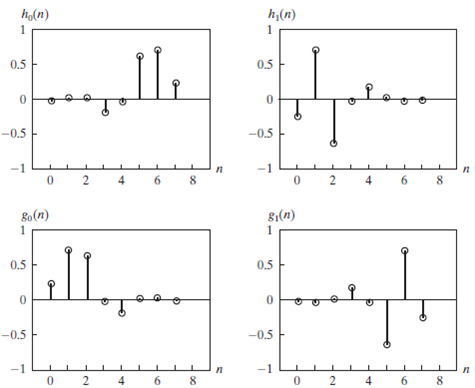
FIGURE 7.5 Six functionally related filter impulse responses: (a) reference response; (b) sign reversal; (c) and (d) order reversal (differing by the delay introduced); (e) modulation; and (f) order reversal and modulation.

TABLE 7.1 Daubechies 8-tap orthonormal filter coefficients for g0(n)(Daubechies [1992]).

FIGURE 7.9 A four-band split of the vase in Fig. 7.1 using the subband coding system of Fig. 7.7. The four subbands that result are the (a) approximation, (b) horizontal detail, (c) vertical detail, and (d) diagonal detail subbands.

both biorthogonal (they satisfy Eq. 7.1-12) and orthonormal (they satisfy Eq. 7.1-13). As a result, the Daubechies 8-tap filters in Fig. 7.8 support error-free reconstruction of the decomposed input.

(7.1-12)

(7.1-13)

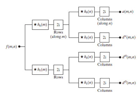
A four-band split of the 512 × 512 image of a vase in Fig. 7.1, based on the filters in Fig. 7.8, is shown in Fig. 7.9. Each quadrant of this image is a subband of size 256 × 256. Beginning with the upper-left corner and proceeding in a clockwise manner, the four quadrants contain approximation subband a, horizontal detail subband dH, diagonal detail subband dD, and vertical detail sub-band dV, respectively. All subbands, except the approximation subband in Fig. 7.9(a), have been scaled to make their underlying structure more visible. Note the visual effects of aliasing that are present in Figs. 7.9(b) and (c)—the dH and dV subbands. The wavy lines in the window area are due to the downsam-pling of a barely discernable window screen in Fig. 7.1. Despite the aliasing, the original image can be reconstructed from the subbands in Fig. 7.9 without error. The required synthesis filters, g0(n)and g1(n), are determined from Table 7.1 and Eq. (7.1-14), and incorporated into a filter bank that roughly mirrors the system in Fig. 7.7. In the new filter bank, filters hi(n)for i = {0, 1} are replaced by their gi(n) counterparts, and upsamplers and summers are added.

(7.1-14)

FIGURE 7.7 A twodimensional, Fourband filter bank for subband image coding.