Consider the competitive market for halogen lamps. The following graph shows the marginal cost (MC)
4. Deriving the short-run supply curve
Consider the competitive market for halogen lamps. The following graph shows the marginal cost (MC), average total cost (ATC), and average variable cost (AVC) curves for a typical firm in the industry.

For each price in the following table, use the graph to determine the number of lamps this firm would produce in order to maximize its profit. Assume that when the price is exactly equal to the average variable cost, the firm is indifferent between producing zero lamps and the profit-maximizing quantity. Also, indicate whether the firm will produce, shut down, or be indifferent between the two in the short run. Lastly, determine whether it will make a profit, suffer a loss, or break even at each price.

On the following graph, use the orange points (square symbol) to plot points along the portion of the firm's short-run supply curve that corresponds to prices where there is positive output. (Note: You are given more points to plot than you need.)

Suppose there are 9 firms in this industry, each of which has the cost curves previously shown.
On the following graph, use the orange points (square symbol) to plot points along the portion of the industry's short-run supply curve that corresponds to prices where there is positive output. (Note: You are given more points to plot than you need.) Then, place the black point (plus symbol) on the graph to indicate the short-run equilibrium price and quantity in this market.
Note: Dashed drop lines will automatically extend to both axes.

At the current short-run market price, firms will _______ in the short run. In the long run, _______ .
Homework Answers
| P | Q | P/S | P/L |
| 4 | 0 | S | L |
| 8 | 0 | S | L |
| 12 | Either 0 or 36000 | Either P or S | L |
| 36 | 48000 | P | Breakeven |
| 48 | 52000 | P | P |
| 60 | 56000 | P | P |
The first graph is correct
When there are 9 firms
| P | Q | S-9 FIRMS |
| 4 | 0 | 0 |
| 8 | 0 | 0 |
| 12 | 36000 | 324000 |
| 36 | 48000 | 432000 |
| 48 | 52000 | 468000 |
| 60 | 56000 | 504000 |
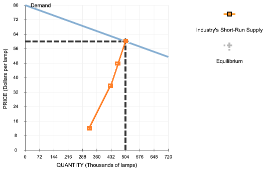
Blanks-
1) produce
2) some firms will enter
Add Answer to:
Consider the competitive market for halogen lamps. The following graph shows the marginal cost (MC)
Consider the competitive market for halogen lamps. The following graph shows the marginal cost (MC), average total cost (ATC), and average variable cost (AVC) curves for a typical firm in the industry.
 Consider the competitive market for halogen lamps. The following graph shows the marginal cost (MC), average total cost (ATC), and average variable cost (AVC) curves for a typical firm in the industry. For each price in the following table, use the graph to determine the number of lamps this firm would produce in order to maximize its profit. Assume that when the price is exactly equal to the average variable cost, the firm is indifferent between producing zero lamps and the...
6. Deriving the short-run supply curve Consider the competitive market for halogen lamps. The following graph...
 6. Deriving the short-run supply curve Consider the competitive market for halogen lamps. The following graph shows the marginal cost (MC), average total cost (ATC), and average variable cost (AVC) curves for a typical firm in the industry. For each price in the following table, use the graph to determine the number of lamps this firm would produce in order to maximize its profit. Assume that when the price is exactly equal to the average variable cost, the firm is indifferent between...
Deriving the short-run supply curve Consider the competitive market for halogen lamps. The following graph shows...
 Deriving the short-run supply curve
Consider the competitive market for halogen lamps. The following
graph shows the marginal cost (MC), average total cost (ATC), and
average variable cost (AVC) curves for a typical firm in the
industry.
For each price in the following table, use the graph to
determine the number of lamps this firm would produce in order to
maximize its profit. Assume that when the price is exactly equal to
the average variable cost, the firm is indifferent...
Deriving the short-run supply curve
Consider the competitive market for halogen lamps. The following
graph shows the marginal cost (MC), average total cost (ATC), and
average variable cost (AVC) curves for a typical firm in the
industry.
For each price in the following table, use the graph to
determine the number of lamps this firm would produce in order to
maximize its profit. Assume that when the price is exactly equal to
the average variable cost, the firm is indifferent...
Consider the perfectly competitive market for sports jackets. The following graph shows the marginal cost (MC),...
 Consider the perfectly competitive market for sports jackets. The following graph shows the marginal cost (MC), average total cost (ATC), and average variable cost (AVC) curves for a typical firm in the industry. For each price in the following table, use the graph to determine the number of jackets this firm would produce in order to maximize its profit. Assume that when the price is exactly equal to the average variable cost, the firm is indifferent between producing zero jackets and...
17. Deriving the short-run supply curve Consider the competitive market for dress shirts. The following graph shows the marginal cost (MC)
 17. Deriving the short-run supply curve Consider the competitive market for dress shirts. The following graph shows the marginal cost (MC), average total cost (ATC), and average variable cost (AVC) curves for a typical firm in the industry. For each price in the following table, use the graph to determine the number of shirts this firm would produce in order to maximize its profit. Assume that when the price is exactly equal to the average variable cost, the firm is indifferent between...
6. Deriving the short-run supply curve Consider the competitive market for halogen lamps. The following graph...
 6. Deriving the short-run supply curve Consider the competitive market for halogen lamps. The following graph shows the marginal cost (MC), average total cost (ATC), and average variable cost (AVC) curves for a typical firm in the industry. COSTS (Dollars) AVC МСП OHH 0 10 90 100 20 30 40 50 60 70 80 QUANTITY (Thousands of lamps) On the following graph, use the orange points (square symbol) to plot points along the portion of the firm's short-run supply curve...
6. Deriving the short-run supply curve Consider the competitive market for halogen lamps. The following graph...
 6. Deriving the short-run supply curve Consider the competitive market for halogen lamps. The following graph shows the marginal cost (MC), average total cost (ATC), and average variable cost (AVC) curves for a typical firm in the industry. ATC COSTS (Dollars) MC D 0 + 0 + + + + + 20 30 40 50 60 70 80 QUANTITY (Thousands of lamps) + 90 10 100 For each price in the following table, use the graph to determine the number...
Consider the competitive market for dress shirts. The foflowinggrapit shows the marginal cost (MC), average...
 Consider the competitive market for dress shirts. The following
graphic shows the marginal cost (MC), average total cost (ATC) , and
average variable cost (AVC) curves for a typical industry For each price in the following table, use the graph to determine the number of shirts this firm would produce in order to maximize its profit. Assume that when the price is exactly equal to the average variable cost, the firm is Indifferent between producing zero shirts and the profit-maximizing quantity....
Consider the competitive market for dress shirts. The following
graphic shows the marginal cost (MC), average total cost (ATC) , and
average variable cost (AVC) curves for a typical industry For each price in the following table, use the graph to determine the number of shirts this firm would produce in order to maximize its profit. Assume that when the price is exactly equal to the average variable cost, the firm is Indifferent between producing zero shirts and the profit-maximizing quantity....
Consider the perfectly competitive market for halogen ceiling lamps. The following graph shows the marginal cost...
 Consider the perfectly competitive market for halogen ceiling lamps. The following graph shows the marginal cost (MC), average total cost (ATC), and average variable cost (AVC) curves for a typical firm in the industry. COSTS (Dollars per tamp) 100 MC 90 80 70 60 50 ATC AVC 40 30 20 10 0 5 10 15 20 25 30 35 40 45 50 QUANTITY OF OUTPUT (Thousands of lamps) For each price in the following table, use the graph to determine...
Consider the competitive market for dress shirts. The following graph shows the marginal cost (MC), average...
 Consider the competitive market for dress shirts. The following
graph shows the marginal cost (MC), average total cost (ATC), and
average variable cost (AVC) curves for a typical firm in the
industry.
On the following graph, use the orange points (square
symbol) to plot points along the portion of the
firm's short-run supply curve that corresponds to
prices where there is positive output. (Note: You
are given more points to plot than you need.)
At the current short-run market price,...
Consider the competitive market for dress shirts. The following
graph shows the marginal cost (MC), average total cost (ATC), and
average variable cost (AVC) curves for a typical firm in the
industry.
On the following graph, use the orange points (square
symbol) to plot points along the portion of the
firm's short-run supply curve that corresponds to
prices where there is positive output. (Note: You
are given more points to plot than you need.)
At the current short-run market price,...
 Deriving the short-run supply curve
Consider the competitive market for halogen lamps. The following
graph shows the marginal cost (MC), average total cost (ATC), and
average variable cost (AVC) curves for a typical firm in the
industry.
For each price in the following table, use the graph to
determine the number of lamps this firm would produce in order to
maximize its profit. Assume that when the price is exactly equal to
the average variable cost, the firm is indifferent...
Deriving the short-run supply curve
Consider the competitive market for halogen lamps. The following
graph shows the marginal cost (MC), average total cost (ATC), and
average variable cost (AVC) curves for a typical firm in the
industry.
For each price in the following table, use the graph to
determine the number of lamps this firm would produce in order to
maximize its profit. Assume that when the price is exactly equal to
the average variable cost, the firm is indifferent...
 6. Deriving the short-run supply curve Consider the competitive market for halogen lamps. The following graph shows the marginal cost (MC), average total cost (ATC), and average variable cost (AVC) curves for a typical firm in the industry. COSTS (Dollars) AVC МСП OHH 0 10 90 100 20 30 40 50 60 70 80 QUANTITY (Thousands of lamps) On the following graph, use the orange points (square symbol) to plot points along the portion of the firm's short-run supply curve...
 6. Deriving the short-run supply curve Consider the competitive market for halogen lamps. The following graph shows the marginal cost (MC), average total cost (ATC), and average variable cost (AVC) curves for a typical firm in the industry. ATC COSTS (Dollars) MC D 0 + 0 + + + + + 20 30 40 50 60 70 80 QUANTITY (Thousands of lamps) + 90 10 100 For each price in the following table, use the graph to determine the number...
 Consider the perfectly competitive market for halogen ceiling lamps. The following graph shows the marginal cost (MC), average total cost (ATC), and average variable cost (AVC) curves for a typical firm in the industry. COSTS (Dollars per tamp) 100 MC 90 80 70 60 50 ATC AVC 40 30 20 10 0 5 10 15 20 25 30 35 40 45 50 QUANTITY OF OUTPUT (Thousands of lamps) For each price in the following table, use the graph to determine...
 Consider the competitive market for dress shirts. The following
graph shows the marginal cost (MC), average total cost (ATC), and
average variable cost (AVC) curves for a typical firm in the
industry.
On the following graph, use the orange points (square
symbol) to plot points along the portion of the
firm's short-run supply curve that corresponds to
prices where there is positive output. (Note: You
are given more points to plot than you need.)
At the current short-run market price,...
Consider the competitive market for dress shirts. The following
graph shows the marginal cost (MC), average total cost (ATC), and
average variable cost (AVC) curves for a typical firm in the
industry.
On the following graph, use the orange points (square
symbol) to plot points along the portion of the
firm's short-run supply curve that corresponds to
prices where there is positive output. (Note: You
are given more points to plot than you need.)
At the current short-run market price,...
Most questions answered within 3 hours.
-
Two small plastic spheres are given positive electrical charges.
When they are a distance of 15.4...
asked 4 minutes ago -
An acidic solution containing gold ions is
electrolyzed, producing gaseous oxygen (from water) at the anode...
asked 19 minutes ago -
Assume that the population of Mexico is 128
million and that the population increases 1.01
percentannually....
asked 1 hour ago -
Can someone please help me add appropriate descriptive
comments to each line of code in the...
asked 1 hour ago -
Romeo wishes to throw a bouquet of flowers to Juliet, who is on
a second-story balcony,...
asked 2 hours ago -
Why is QE a controversial monetary policy tool.
A. It may lead to excessive inflation.B. By...
asked 2 hours ago -
Principles of Programming midterm study guide help!
1.)
______ Which of the following would reference the...
asked 2 hours ago -
A finite potential well has depth U0 = 2.78 eV . What is the
penetration distance...
asked 3 hours ago -
1. The bus bars of a power station are in two sections A and B
separated...
asked 3 hours ago -
Fiscal policy is the deliberate manipulation of taxes and
government spending to alter GDP, employment, inflation...
asked 3 hours ago -
evaluating an expression using only one digit and + and - as
operators ....3+5-1+7-5+8
-----------------------
stack...
asked 3 hours ago -
Two concentric current loops lie in the same plane. The smaller
loop has a radius of...
asked 4 hours ago