
Homework Answers
(a)Supply curve for a perfectly competitive firm is the marginal cost curve above AVC curve
.At P=2 the MC=AVC, so from P=2 the supply curve of a firm will start.
We have to draw market supply curve and we know there are 100 firms. At price level of 2 each firm supply 2 units so 100 firms will supply 200 units. At price level 3 each firm supply 3 units so 100 firms will supply 300 units. Similarly, for rest of the units we can find market supply and joining the points we get market supply curve.
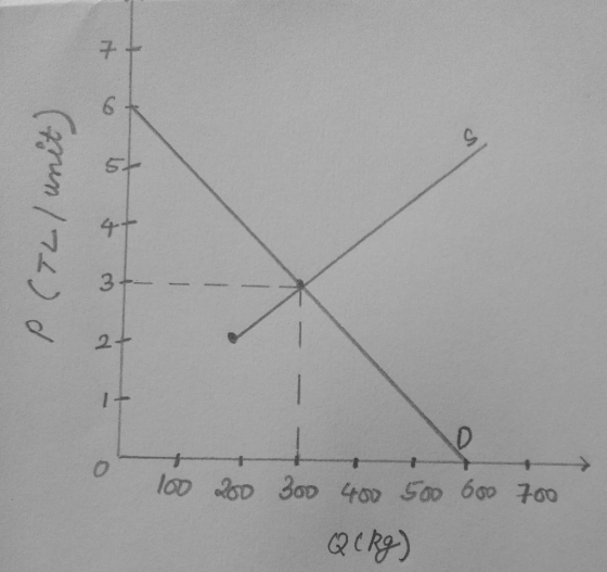
(b) Market price and quantity, we get from the intersection of market supply and market demand curve.
So, market price is 3 and market quantity is 300. There are 100 firms so quantity supplied by each firm is 3.
(c) To find whether firm is making loss or profit we will have to draw individual demand and marginal revenue curve on the right-hand side graph which is given by the equilibrium price of 3. We see that at equilibrium price level 3 and quantity 3 the ATC curve is above price level. Area below MR curve is total revenue and area below ATC is total cost. At equilibrium quantity of 3 the total cost exceeds total revenue so firm is making loss.
 (d) As existing firm is making
loss so there will be exit of firm from the industry. This exit
will continue till price equals ATC and firms are in long run
making zero profit.
(d) As existing firm is making
loss so there will be exit of firm from the industry. This exit
will continue till price equals ATC and firms are in long run
making zero profit.
(e) We can see from left hand diagram that at P=4 the market demand for apples fall to Q=200. At P=4 the quantity supplied by each firm is 4. So, the number of firms producing in long run will be 50 firms (i.e. 200/4).

Add Answer to:
14. (Perfect Competition) Apples are produced in a perfectly competitive industry. As- sume that there are...
Question: These diagrams, pertain to a perfectly competitive firm producing output q and the industry in...
 Question: These diagrams, pertain to a perfectly competitive firm producing output q and the industry in which it operates. What should we expect in the long run on the number of firms, market supply and equilibrium price? MC ATC AVC MR P
The long-run supply curve for a perfectly competitive, constant-cost industry O is horizontal at minimum ATC....
 The long-run supply curve for a perfectly competitive, constant-cost industry O is horizontal at minimum ATC. O is upward-sloping. O is horizontal at minimum AVC. O is found by adding up the marginal cost curves for all firms in the industry. As more firms enter the market: O the short-run market demand curve shifts to the left. O the short-run market supply curve shifts to the right. O the short-run market supply curve shifts to the left. O the short-run...
Consider a perfectly competitive market for titanium. Assume that all firms in the industry are identical and...
 Consider a perfectly competitive market for titanium. Assume that all firms in the industry are identical and have the marginal cost (MC), average total cost (ATC), and average variable cost (AVC) curves shown on the following graph. Assume also that it does not matter how many firms are in the industry Tool Tip: Place the mouse cursor over orange square points on the MC curve to see coordinates. COST PER UNIT IDollars per pound) 10 MC ATC AVC 0 5...
Problem 1. (13 points) Markets: Perfect Competition. Assume that a perfectly competitive, constant cost industry is...
Problem 1. (13 points) Markets: Perfect Competition. Assume that a perfectly competitive, constant cost industry is in a long run equilibrium with 35 firms. Each firm is producing 90 units of output which it sells at the price of $39 per unit; out of this amount each firm is paying $5 tax per unit of the output. The government decides to decrease the tax, so the firms will be paying $3 tax per unit. a) Explain what would happen in...
For a perfectly competitive market made up of firms represented in the graph below, what is...
 For a perfectly competitive market made up of firms represented in the graph below, what is the long run equilibrium price of the good? Cost ($) MC ATC AVC $16 $14 $12 $10 Quantity $14 $10 $12 $16 For a perfectly competitive market made up of firms represented in the graph below, if the price is $14, Cost ($) MC ATC $16 AVC - $14 $12 $10 Quantity The firm is operating at its minimum long run average total cost....
Аа Аа Consider a perfectly competitive market for titanium. Assume that all firms in the industry...
 Аа Аа Consider a perfectly competitive market for titanium. Assume that all firms in the industry are identical and have the marginal cost (MC), average total cost (ATC), and average variable cost (AVC) curves shown on the following graph. Assume also that it does not matter how many firms are in the industry. Tool Tip: Place the mouse cursor over orange square points on the MC curve to see coordinates. COSTS Dollars per pound) 10 MC 9 8 7 ATC...
3. Perfect Competition Market (Total 8 points) a. For a perfectly competitive firm, illustrate a case...
 3. Perfect Competition Market (Total 8 points) a. For a perfectly competitive firm, illustrate a case where the firm is facing PMC SRATC LRATC by using yin the following diagram. In this diagram, you should include demand curve (d), marginal cost curve (MC), short run average total cost curve (SRATC), and long run average total cost curve (LRATC). Remember to label all axes. (2 points) pves vwerase totail cost curve (SRATC,aushould include demandcun b. Does the firm exhibit productive efficiency?...
6. Short-run perfectly competitive equilibrium Consider a perfectly competitive market for wheat in Philadelphia. There...
 6. Short-run perfectly competitive equilibrium Consider a perfectly competitive market for wheat in Philadelphia. There are 80 firms in the industry, each of which has the cost curves shown on the following graph: MC ATC COST (Cents per bushel) AVC 0 5 10 15 20 25 30 35 40 45 50 Demand Supply Curve Equilibrium PRICE (Cents per bushel) 0 400 800 1200 1600 2000 2400 2800 3200 3600 4000 QUANTITY OF OUTPUT (Thousands of bushels) in the short run....
71:06 supply and long-run equillbrium i Consider a perfectly competitive market for titanium. Ass...
 super positive i did this wrong. please help.
71:06 supply and long-run equillbrium i Consider a perfectly competitive market for titanium. Assume that all firms in the industry are identical and have the marginal cost (MC), average total cost (ATC), and average variable cost (AVC) curves shown on the following graph. Assume also that it does not matter how many firms are in the industry Tool Tip: Place the mouse cursor over orange square points on the MC curve to...
super positive i did this wrong. please help.
71:06 supply and long-run equillbrium i Consider a perfectly competitive market for titanium. Assume that all firms in the industry are identical and have the marginal cost (MC), average total cost (ATC), and average variable cost (AVC) curves shown on the following graph. Assume also that it does not matter how many firms are in the industry Tool Tip: Place the mouse cursor over orange square points on the MC curve to...
5. Short-run supply and long-run equilibrium Consider the perfectly competitive market for steel. Assume that, regardless...
 5. Short-run supply and long-run equilibrium Consider the perfectly competitive market for steel. Assume that, regardless of how many firms are in the industry, every firm in the industry is identical and faces the marginal cost (MC), average total cost (ATC), and average variable cost (AVC) curves shown on the following graph. COSTS (Dollars per ton) + MC D AVC 0 10 90 100 20 30 40 50 60 70 80 QUANTITY (Thousands of tons) The following diagram shows the...
 Question: These diagrams, pertain to a perfectly competitive firm producing output q and the industry in which it operates. What should we expect in the long run on the number of firms, market supply and equilibrium price? MC ATC AVC MR P
 The long-run supply curve for a perfectly competitive, constant-cost industry O is horizontal at minimum ATC. O is upward-sloping. O is horizontal at minimum AVC. O is found by adding up the marginal cost curves for all firms in the industry. As more firms enter the market: O the short-run market demand curve shifts to the left. O the short-run market supply curve shifts to the right. O the short-run market supply curve shifts to the left. O the short-run...
 Consider a perfectly competitive market for titanium. Assume that all firms in the industry are identical and have the marginal cost (MC), average total cost (ATC), and average variable cost (AVC) curves shown on the following graph. Assume also that it does not matter how many firms are in the industry Tool Tip: Place the mouse cursor over orange square points on the MC curve to see coordinates. COST PER UNIT IDollars per pound) 10 MC ATC AVC 0 5...
 For a perfectly competitive market made up of firms represented in the graph below, what is the long run equilibrium price of the good? Cost ($) MC ATC AVC $16 $14 $12 $10 Quantity $14 $10 $12 $16 For a perfectly competitive market made up of firms represented in the graph below, if the price is $14, Cost ($) MC ATC $16 AVC - $14 $12 $10 Quantity The firm is operating at its minimum long run average total cost....
 Аа Аа Consider a perfectly competitive market for titanium. Assume that all firms in the industry are identical and have the marginal cost (MC), average total cost (ATC), and average variable cost (AVC) curves shown on the following graph. Assume also that it does not matter how many firms are in the industry. Tool Tip: Place the mouse cursor over orange square points on the MC curve to see coordinates. COSTS Dollars per pound) 10 MC 9 8 7 ATC...
 3. Perfect Competition Market (Total 8 points) a. For a perfectly competitive firm, illustrate a case where the firm is facing PMC SRATC LRATC by using yin the following diagram. In this diagram, you should include demand curve (d), marginal cost curve (MC), short run average total cost curve (SRATC), and long run average total cost curve (LRATC). Remember to label all axes. (2 points) pves vwerase totail cost curve (SRATC,aushould include demandcun b. Does the firm exhibit productive efficiency?...
 6. Short-run perfectly competitive equilibrium Consider a perfectly competitive market for wheat in Philadelphia. There are 80 firms in the industry, each of which has the cost curves shown on the following graph: MC ATC COST (Cents per bushel) AVC 0 5 10 15 20 25 30 35 40 45 50 Demand Supply Curve Equilibrium PRICE (Cents per bushel) 0 400 800 1200 1600 2000 2400 2800 3200 3600 4000 QUANTITY OF OUTPUT (Thousands of bushels) in the short run....
 super positive i did this wrong. please help.
71:06 supply and long-run equillbrium i Consider a perfectly competitive market for titanium. Assume that all firms in the industry are identical and have the marginal cost (MC), average total cost (ATC), and average variable cost (AVC) curves shown on the following graph. Assume also that it does not matter how many firms are in the industry Tool Tip: Place the mouse cursor over orange square points on the MC curve to...
super positive i did this wrong. please help.
71:06 supply and long-run equillbrium i Consider a perfectly competitive market for titanium. Assume that all firms in the industry are identical and have the marginal cost (MC), average total cost (ATC), and average variable cost (AVC) curves shown on the following graph. Assume also that it does not matter how many firms are in the industry Tool Tip: Place the mouse cursor over orange square points on the MC curve to...
 5. Short-run supply and long-run equilibrium Consider the perfectly competitive market for steel. Assume that, regardless of how many firms are in the industry, every firm in the industry is identical and faces the marginal cost (MC), average total cost (ATC), and average variable cost (AVC) curves shown on the following graph. COSTS (Dollars per ton) + MC D AVC 0 10 90 100 20 30 40 50 60 70 80 QUANTITY (Thousands of tons) The following diagram shows the...
Most questions answered within 3 hours.
-
1- What is the energy of a photon with a frequency of 7.01 ×
10¹⁴ s⁻¹?...
asked 12 minutes ago -
Cesar needs to make a decision whether to fertilize his garden
or not. His profit depends...
asked 15 minutes ago -
Illustrate the Substitution Effect, Income Effect and Total
Effect of a normal good and an inferior...
asked 14 minutes ago -
Your company has six-sigma conformance for each of 10 component
that are a part if a...
asked 28 minutes ago -
Explain the buffering components of urine, the chemical
equation, where the system is found and find...
asked 33 minutes ago -
The financial records of Leon Paul Inc. were destroyed by fire
at the end of 2017....
asked 35 minutes ago -
The normal-curve approximation can also be used for discrete
distribution other than the binomial distribution. For...
asked 1 hour ago -
1. Find the following z values for the standard normal
variable Z. (You may find it...
asked 1 hour ago -
Lakeside Motors will sell you a $9000 car for $225 a month for 60
months. What...
asked 52 minutes ago -
how immigrants foster innovations and how it lead to economic
growth of the host country????
"Not...
asked 1 hour ago -
What are some of the methods that creditors use to
reduce risk in credit transactions?
asked 57 minutes ago -
1 Explain HOW you would use the scientific method to test
which helps kids lose weight:...
asked 1 hour ago