Question

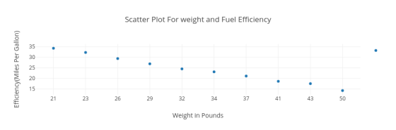
Directions: There are THREE questions on this take home quiz along with one extra credit ques- tion. Carefully write up your answers (and work) to the following questions on a SEPARATE piece of paper. You may work with up to two other people. Make sure that if you do choose to work in a group, you submit only one set of answers with all of your names on it. Since this is a take-home assignment you may talk with other students and use any other resources you wish. Due: In class Monday July 1st Question 1) Suppose you're interested in studying the relationship between the weight of a non- hybrid/electric car and the miles per gallon the car gets. To do this you take a random sample of 10 non-hybrid/electric cars and record their weight in hundreds of pounds and their fuel efficiency in miles per gallon. (Note: Make you sure you pay special attention to the units in this problem) You get the following data: Fuel Efficiency in Miles Per Gallon Weight in Hundreds of Pounds 21 34.3 23 32.3 26 29.4 29 26.9 32 24.5 34 23.1 37 21.1 41 18.6 43 17.5 50 14.2 to label your axes. (a) Draw a scatterplot for this data. Make sure (b) Calculate the correlation coefficient, and decide if there is enough evidence for a correlation (c) Construct the LSR for this data. Make sure to keep at least two decimal places for both your slope and y-intercept (d) Graph the LSR on your scatterplot (e) Interpret the slope of the LSR (f) Interpret the intercept of the LSR. (g) Calculate and interpret the coefficient of determination. (h) What does your model predict for the fuel efficiency of a car that weighs 4000 pounds? Would you trust this prediction? (0) Construct the residual plot for this data. Is a linear model appropriate? Why or why not?

Answer 1

a)

Scatter Plot For weight and Fuel Efficiency 35 30 25 20 15 50 43 41 37 34 32 29 Weight in Pounds 26 23 21 Efficlency(Miles Per Gallon)

b)

Data is:

Weight(X)	Efficiency(Y)
21	34.3
23	32.3
26	29.4
29	26.9
32	24.5
34	23.1
37	21.1
41	18.6
43	17.5
50	14.2

X Values
Sum = 336

n = 10

Mean = 33.6
$\sum$ (X - M_x)² = SS_x = 776.4

(X - Mx)2 158.76
112.36
57.76
21.16
2.56
0.16
11.56
54.76
88.36
268.96
Sum: 776.400

Y Values
Sum = 241.9
Mean = 24.19
$\sum$ (Y - M_y)² = SS_y = 389.109

(Y - M_y)²

102.212
65.772
27.144
7.344
0.096
1.188
9.548
31.248
44.756
99.800

Sum: 389.109

X and Y combined

N = 10
$\sum$ (X - M_x)(Y - M_y) = -544.94

(X - M_x)(Y - M_y)

-127.386
-85.966
-39.596
-12.466
-0.496
-0.436
-10.506
-41.366
-62.886
-163.836

Sum: - 544.940

R Calculation
r = ∑((X - M_y)(Y - M_x)) / √((SS_x)(SS_y))

r = -544.94 / √((776.4)(389.109)) = -0.9914

There exists a very strong correlation between Weights and Fuel Efficiency. The relationship is negative. If the weight increases Fuel Efficiency Decreases.

c)

Calcualting the Linear Regression equation between Weight and Fuel Efficiency using excel we get below results:

SUMMARY OUTPUT
Regression Statistics
Multiple R	0.991448788
R Square	0.982970698
Adjusted R Square	0.980842036
Standard Error	0.910099892
Observations	10
ANOVA
	df	SS	MS	F	Significance F
Regression	1	382.4827455	382.4827455	461.7785146	2.3154E-08
Residual	8	6.626254508	0.828281813
Total	9	389.109
	Coefficients	Standard Error	t Stat	P-value	Lower 95%	Upper 95%	Lower 95.0%	Upper 95.0%
Intercept	47.77318393	1.134561285	42.10718676	1.11514E-10	45.15688091	50.38948694	45.15688091	50.38948694
Weight(X)	-0.701880474	0.032662265	-21.48903243	2.3154E-08	-0.777199792	-0.626561156	-0.777199792	-0.626561156

Thus, equation becomes,

Fuel Efficiency(Y) = 47.77 - 0.701 * X

Now, predicting the value of efficiency using this equation we get

Weight(X)	Efficiency(Y)	Predicted(Y)
21	34.3	33.049
23	32.3	31.647
26	29.4	29.544
29	26.9	27.441
32	24.5	25.338
34	23.1	23.936
37	21.1	21.833
41	18.6	19.029
43	17.5	17.627
50	14.2	12.72

d)

The Linear Predicted values on our scatter plot is shown below:

Linear Plot For weight and Predicted Fuel Efficiency Linear Predicted values trace1 40 30 20 10 40 20 30 50 60 Weight in Pounds Predicted Efficlency(Miles Per Gallon) 10

As per HomeworkLib policy we need to solve four sub parts per question. Please post the remaining questions in another post.