
Homework Answers
![As n gets large,fw Cumulative dirty bron function of sin」 well approni mahed bt tne Normal [0,1] Cumulanve. dlisri bution -fu](http://img.homeworklib.com/questions/d6805e90-ada6-11ea-917a-e5dbe6930bf9.png?x-oss-process=image/resize,w_560)

Add Answer to:
L.9) Central Limit Theorem Central Limit Theorem Version 1 says Go with independent random variables (Xi,...
1. Give the experimental line a real test. Come up with an n so that if...
 1. Give the experimental line a real test. Come up with an n so
that if the experimental line produces n chips with failure rate
6/38 or less, then the probability of getting a failure rate 6/38
or less under the original production system is less than 0.01.
2. If two random variables have the same generating function,
must they have the same cumulative distribution function?
L.9) Central Limit Theorem Central Limit Theorem Version 1 says Go with independent random...
1. Give the experimental line a real test. Come up with an n so
that if the experimental line produces n chips with failure rate
6/38 or less, then the probability of getting a failure rate 6/38
or less under the original production system is less than 0.01.
2. If two random variables have the same generating function,
must they have the same cumulative distribution function?
L.9) Central Limit Theorem Central Limit Theorem Version 1 says Go with independent random...
If two random variables have the same generating function, must they have the same cumulative distribution...
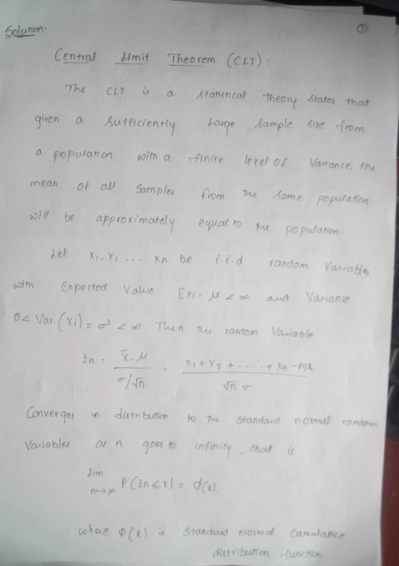
 If two random variables have the same generating function, must they have the same cumulative distribution function? L.8) Central Limit Theorem One version of Central Limit Theorem says this: Go with independent random variables (Xi, X2, X3, ..., X.....] all with the same cumulative distribution function so that: 11-Expect[Xi]-Expect[s] and σ. varpk-VarX] for all i and j . Put: s[n] = As n gets large, the cumulative distribution function of S[n] is well approximated by the Normal[o, 1] cumulative distribution...
Central Limit Theorem: let x1,x2,...,xn be I.I.D. random variables with E(xi)= U Var(xi)= (sigma)^2 defind Z=...
Central Limit Theorem: let x1,x2,...,xn be I.I.D. random variables with E(xi)= U Var(xi)= (sigma)^2 defind Z= x1+x2+...+xn the distribution of Z converges to a gaussian distribution P(Z<=z)=1-Q((z-Uz)/(sigma)^2) Use MATLAB to prove the central limit theorem. To achieve this, you will need to generate N random variables (I.I.D. with the distribution of your choice) and show that the distribution of the sum approaches a Guassian distribution. Plot the distribution and matlab code. Hint: you may find the hist() function helpful
R commands 2) Illustrating the central limit theorem. X, X, X, a sequence of independent random variables with the same distribution as X. Define the sample mean X by X = A + A 2 be a random va...
 R commands
2) Illustrating the central limit theorem. X, X, X, a sequence of independent random variables with the same distribution as X. Define the sample mean X by X = A + A 2 be a random variable having the exponential distribution with A -2. Denote by -..- The central limit theorem applied to this particular case implices that the probability distribution of converges to the standard normal distribution for certain values of u and o (a) For what...
R commands
2) Illustrating the central limit theorem. X, X, X, a sequence of independent random variables with the same distribution as X. Define the sample mean X by X = A + A 2 be a random variable having the exponential distribution with A -2. Denote by -..- The central limit theorem applied to this particular case implices that the probability distribution of converges to the standard normal distribution for certain values of u and o (a) For what...
The central limit theorem says that when a simple random sample of size n is drawn...
The central limit theorem says that when a simple random sample of size n is drawn from any population with mean μ and standard deviation σ, then when n is sufficiently large the distribution of the sample mean is approximately Normal. the standard deviation of the sample mean is σ2nσ2n. the distribution of the sample mean is exactly Normal. the distribution of the population is approximately Normal.
,X, ,n. independent, the central Xi, E(X)=0, var(X)-σ are Prove 3. Assume <o。 13<oo, 1=1, limit...
 ,X, ,n. independent, the central Xi, E(X)=0, var(X)-σ are Prove 3. Assume <o。 13<oo, 1=1, limit theorem (CLT) based EX1 result regarding what are conditions on σ that we need to assume in order for the x.B.= Σσ, as n →oo. In this context, X,, B" =y as n →oo, In this context, result to hold?
Law of Large Number↓ Led tin eperaje Theorem 9.11. (Central limit theorem) Suppose that we have...
 Law of Large Number↓
Led tin eperaje Theorem 9.11. (Central limit theorem) Suppose that we have i.i.d. random variables Xi,X2. X3,... with finite mean EX and finite variance Var(X) = σ2. Let Sn-Xi + . . . + Xn. Then for any fixed - oo<a<b<oo we have lim Pax (9.6) Theorem 4.8. (Law of large numbers for binomial random variables) For any fixed ε > 0 we have (4.7) n-00
Law of Large Number↓
Led tin eperaje Theorem 9.11. (Central limit theorem) Suppose that we have i.i.d. random variables Xi,X2. X3,... with finite mean EX and finite variance Var(X) = σ2. Let Sn-Xi + . . . + Xn. Then for any fixed - oo<a<b<oo we have lim Pax (9.6) Theorem 4.8. (Law of large numbers for binomial random variables) For any fixed ε > 0 we have (4.7) n-00
L.1) BinomialDist[1, p] random variables In what context do random variables with BinomialDist[1, p] arise? L.2)...
 L.1) BinomialDist[1, p] random variables In what context do random variables with BinomialDist[1, p] arise? L.2) Expected value and Variance for the Binomial[1, p] and Binomial[n, p] random variables a) Go with a random variable X with BinomialDist[1, p Calculate Expect[X] and Var[X]. b) Go with a random variable X with BinomialDist[n, p]. Use the fact that X is the sum of n independent random variables each with BinomialDist[1, pl to explain why: Expect[x]-n p and Var[X]-np(p) L.3) Relations among...
1. The random variables Xi, X2,.. are independent and identically distributed (iid), each with pdf f given in Assignment 4, Question 1. Let Sn- Xi+.+X Using the Central Limit Theorem and the graph of...
 1. The random variables Xi, X2,.. are independent and identically distributed (iid), each with pdf f given in Assignment 4, Question 1. Let Sn- Xi+.+X Using the Central Limit Theorem and the graph of the standard normal distribution in Figure 1, approximate the probability P(S100 >600). Express your answer in the format x.x-10-x. Verify your answer by simulating 10,000 outcomes of Si00 and counting how many of them are > 600. Show the code 1.00 0.95 0.90 0.85 1.2 1.4...
 1. Give the experimental line a real test. Come up with an n so
that if the experimental line produces n chips with failure rate
6/38 or less, then the probability of getting a failure rate 6/38
or less under the original production system is less than 0.01.
2. If two random variables have the same generating function,
must they have the same cumulative distribution function?
L.9) Central Limit Theorem Central Limit Theorem Version 1 says Go with independent random...
1. Give the experimental line a real test. Come up with an n so
that if the experimental line produces n chips with failure rate
6/38 or less, then the probability of getting a failure rate 6/38
or less under the original production system is less than 0.01.
2. If two random variables have the same generating function,
must they have the same cumulative distribution function?
L.9) Central Limit Theorem Central Limit Theorem Version 1 says Go with independent random...
 If two random variables have the same generating function, must they have the same cumulative distribution function? L.8) Central Limit Theorem One version of Central Limit Theorem says this: Go with independent random variables (Xi, X2, X3, ..., X.....] all with the same cumulative distribution function so that: 11-Expect[Xi]-Expect[s] and σ. varpk-VarX] for all i and j . Put: s[n] = As n gets large, the cumulative distribution function of S[n] is well approximated by the Normal[o, 1] cumulative distribution...
 R commands
2) Illustrating the central limit theorem. X, X, X, a sequence of independent random variables with the same distribution as X. Define the sample mean X by X = A + A 2 be a random variable having the exponential distribution with A -2. Denote by -..- The central limit theorem applied to this particular case implices that the probability distribution of converges to the standard normal distribution for certain values of u and o (a) For what...
R commands
2) Illustrating the central limit theorem. X, X, X, a sequence of independent random variables with the same distribution as X. Define the sample mean X by X = A + A 2 be a random variable having the exponential distribution with A -2. Denote by -..- The central limit theorem applied to this particular case implices that the probability distribution of converges to the standard normal distribution for certain values of u and o (a) For what...
 ,X, ,n. independent, the central Xi, E(X)=0, var(X)-σ are Prove 3. Assume <o。 13<oo, 1=1, limit theorem (CLT) based EX1 result regarding what are conditions on σ that we need to assume in order for the x.B.= Σσ, as n →oo. In this context, X,, B" =y as n →oo, In this context, result to hold?
 Law of Large Number↓
Led tin eperaje Theorem 9.11. (Central limit theorem) Suppose that we have i.i.d. random variables Xi,X2. X3,... with finite mean EX and finite variance Var(X) = σ2. Let Sn-Xi + . . . + Xn. Then for any fixed - oo<a<b<oo we have lim Pax (9.6) Theorem 4.8. (Law of large numbers for binomial random variables) For any fixed ε > 0 we have (4.7) n-00
Law of Large Number↓
Led tin eperaje Theorem 9.11. (Central limit theorem) Suppose that we have i.i.d. random variables Xi,X2. X3,... with finite mean EX and finite variance Var(X) = σ2. Let Sn-Xi + . . . + Xn. Then for any fixed - oo<a<b<oo we have lim Pax (9.6) Theorem 4.8. (Law of large numbers for binomial random variables) For any fixed ε > 0 we have (4.7) n-00
 L.1) BinomialDist[1, p] random variables In what context do random variables with BinomialDist[1, p] arise? L.2) Expected value and Variance for the Binomial[1, p] and Binomial[n, p] random variables a) Go with a random variable X with BinomialDist[1, p Calculate Expect[X] and Var[X]. b) Go with a random variable X with BinomialDist[n, p]. Use the fact that X is the sum of n independent random variables each with BinomialDist[1, pl to explain why: Expect[x]-n p and Var[X]-np(p) L.3) Relations among...
 1. The random variables Xi, X2,.. are independent and identically distributed (iid), each with pdf f given in Assignment 4, Question 1. Let Sn- Xi+.+X Using the Central Limit Theorem and the graph of the standard normal distribution in Figure 1, approximate the probability P(S100 >600). Express your answer in the format x.x-10-x. Verify your answer by simulating 10,000 outcomes of Si00 and counting how many of them are > 600. Show the code 1.00 0.95 0.90 0.85 1.2 1.4...
Most questions answered within 3 hours.
-
A small body of mass m performs small oscillations sliding (no
rolling) along the bottom of...
asked 1 minute ago -
The electric field in the region between two oppositely charged,
parallel, conducting plates has a magnitude...
asked 1 minute ago -
A simple random sample was taken to test the claim that the
population mean is no...
asked 1 hour ago -
A set of length measurements are obtained with the values 165.6
± 0.3, 165.1± 0.4,166.4± 1.0,...
asked 1 hour ago -
1. Which of the following is true about unconscionable
contracts?
a. A term is substantially unconscionable...
asked 15 minutes ago -
A company is interested in estimating the costs of lunch
in their cafeteria. After surveying employees,...
asked 47 minutes ago -
A 0.2m diameter ball with an initial velocity of 8m/s rolls up a
hill without slipping....
asked 30 minutes ago -
I want to redraft the solution, using other words , use your own
words don't copy...
asked 19 minutes ago -
Hyundai Motors is considering threesites—A, B,C —at which to
locate a factory to build its new-model...
asked 21 minutes ago -
Learning Outcomes:
Upon the successful completion of this module, you should
understand the following concepts:
Strategic...
asked 22 minutes ago -
Identify four of the five major types of organizations within
the federal bureaucracy, and give examples...
asked 30 minutes ago -
The following data have been obtained
for the effect of solvent composition on the solubility of...
asked 31 minutes ago