
Homework Answers
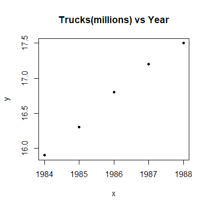
a)
b)
Note that, 
| Serial no. |  |
 |
 |
 |
 |
| 1 | 1984 | 15.9 | 4 | 0.7056 | 1.68 |
| 2 | 1985 | 16.3 | 1 | 0.1936 | 0.44 |
| 3 | 1986 | 16.8 | 0 | 0.0036 | 0 |
| 4 | 1987 | 17.2 | 1 | 0.2116 | 0.46 |
| 5 | 1988 | 17.5 | 4 | 0.5776 | 1.52 |
| Total | 9930 | 83.7 | 10 | 1.692 | 4.1 |
| mean | 1986 | 16.74 |
From the table of calculations above we have

c) The equation of the least square regression is : Y= a+bX
where the least square estimates are as follows, 

Hence ,
Y = -797.52 + 0.41 X is the required equation.
Add Answer to:
3. World truck production (fictional) ON HTAM Year x 1984 1985 1986 1987 1988 15.9 16.3...
3. World truck production (fictional) Year x Trucks y (millions) 1984 15.9 1985 16.3 1986 16.8...
 3. World truck production (fictional) Year x Trucks y (millions) 1984 15.9 1985 16.3 1986 16.8 1987 17.2 1988 17.5 a) Construct a scatterplot (show the rough graph) b) Find the correlation coefficient r c) Find the formula for the regression line
2. Find the five-number summary and construct a boxplot for the following data: 12, 31, 23,...
 2. Find the five-number summary and construct a boxplot for the following data: 12, 31, 23, 8, 23, 11, 33, 17, 28, 23, 23, 16 andro 3. World truck production (fictional) Year x 1984 1985 1986 1987 1988 Trucks y (millions) 15.9 16.3 16.8 17.2 17.5 a) Construct a scatterplot (show the rough graph) 1984 1915 iane 1917 1916 be b) Find the correlation coefficient c) Find the formula for the regression line
1. A survey of the income of 9 students was conducted and the results are shown...
 1. A survey of the income of 9 students was conducted and the results are shown in the table below. 21342 22356 28624 12455 15487 16489 14596 25624 52483 Compute the mean and median of the above data. 2. Find the five-number summary and construct a boxplot for the following data: 12, 31, 23, 8, 23, 11, 33, 17, 28, 23, 23, 16 3. World truck production (fictional) 1985 1986 1987 1988 Year x Trucks y (millions) 1984 15.9 16.3...
5.6 Year 1981 1982 1983 1984 1985 1986 1987 1988 1989 1990 1991 1992 1993 1994...
 5.6 Year 1981 1982 1983 1984 1985 1986 1987 1988 1989 1990 1991 1992 1993 1994 1995 1996 1997 1998 1999 2000 2001 2002 2003 2004 2005 2006 2007 2008 x (L1) y (L2) Inflation Unemployment 8.9 7.6 3.8 9.7 3.8 9.6 3.9 7.5 3.8 7.2 1.1 7 4.4 6.2 4.4 5.5 4.6 5.3 6.1 3.1 6.8 2.9 7.5 2.7 6.9 2.7 6.1 2.5 5.6 3.3 5.4 1.7 4.9 1.6 4.5 2.7 4.2 4 1.6 4.7 2.4 5.8 1.9 6...
Setting k = 3, what is the value of the mean square of errors (Please include calculations/steps) Year X Price Index 1985 1 107.7450408 1986 2 111.1730909 1987 3 118.9245131 1988 4 122.8489601 112.61...
 Setting k = 3, what is the value of the mean square of errors
(Please include calculations/steps)
Year X Price Index 1985 1 107.7450408 1986 2 111.1730909 1987 3 118.9245131 1988 4 122.8489601 112.614215 10.234745 10.234745 104.750009 0.083312 1989 5 127.5113167 117.648855 9.862462 9.862462 97.268157 0.077346 199 6 126.4770851 | 123.09493 3.382155 | 3.382155 | 11.4389731 0.026741 1991 7 116.3061973 125.612454 -9.306257 9.306257 86.606413 0.080015
Year X Price Index 1985 1 107.7450408 1986 2 111.1730909 1987 3 118.9245131 1988 4...
Setting k = 3, what is the value of the mean square of errors
(Please include calculations/steps)
Year X Price Index 1985 1 107.7450408 1986 2 111.1730909 1987 3 118.9245131 1988 4 122.8489601 112.614215 10.234745 10.234745 104.750009 0.083312 1989 5 127.5113167 117.648855 9.862462 9.862462 97.268157 0.077346 199 6 126.4770851 | 123.09493 3.382155 | 3.382155 | 11.4389731 0.026741 1991 7 116.3061973 125.612454 -9.306257 9.306257 86.606413 0.080015
Year X Price Index 1985 1 107.7450408 1986 2 111.1730909 1987 3 118.9245131 1988 4...
A)Determine the correlation coefficient between production budget and box office (dependent variable . .) and interpret...
 A)Determine the correlation coefficient between production budget
and box office (dependent variable . .) and interpret its meaning.
Plot a scatterplot.
B)Find the least squares linear regression equation for production
budget (independent variable) and box office (dependent variable ).
Use the equation to estimate the box office for a movie with a $45
million production budget. Interpret the meaning of the slope and
the y-intercept (be specific using the context provided
here).
Production Number of
Year Picture Studio Box Office...
A)Determine the correlation coefficient between production budget
and box office (dependent variable . .) and interpret its meaning.
Plot a scatterplot.
B)Find the least squares linear regression equation for production
budget (independent variable) and box office (dependent variable ).
Use the equation to estimate the box office for a movie with a $45
million production budget. Interpret the meaning of the slope and
the y-intercept (be specific using the context provided
here).
Production Number of
Year Picture Studio Box Office...
 3. World truck production (fictional) Year x Trucks y (millions) 1984 15.9 1985 16.3 1986 16.8 1987 17.2 1988 17.5 a) Construct a scatterplot (show the rough graph) b) Find the correlation coefficient r c) Find the formula for the regression line
 2. Find the five-number summary and construct a boxplot for the following data: 12, 31, 23, 8, 23, 11, 33, 17, 28, 23, 23, 16 andro 3. World truck production (fictional) Year x 1984 1985 1986 1987 1988 Trucks y (millions) 15.9 16.3 16.8 17.2 17.5 a) Construct a scatterplot (show the rough graph) 1984 1915 iane 1917 1916 be b) Find the correlation coefficient c) Find the formula for the regression line
 1. A survey of the income of 9 students was conducted and the results are shown in the table below. 21342 22356 28624 12455 15487 16489 14596 25624 52483 Compute the mean and median of the above data. 2. Find the five-number summary and construct a boxplot for the following data: 12, 31, 23, 8, 23, 11, 33, 17, 28, 23, 23, 16 3. World truck production (fictional) 1985 1986 1987 1988 Year x Trucks y (millions) 1984 15.9 16.3...
 5.6 Year 1981 1982 1983 1984 1985 1986 1987 1988 1989 1990 1991 1992 1993 1994 1995 1996 1997 1998 1999 2000 2001 2002 2003 2004 2005 2006 2007 2008 x (L1) y (L2) Inflation Unemployment 8.9 7.6 3.8 9.7 3.8 9.6 3.9 7.5 3.8 7.2 1.1 7 4.4 6.2 4.4 5.5 4.6 5.3 6.1 3.1 6.8 2.9 7.5 2.7 6.9 2.7 6.1 2.5 5.6 3.3 5.4 1.7 4.9 1.6 4.5 2.7 4.2 4 1.6 4.7 2.4 5.8 1.9 6...
 Setting k = 3, what is the value of the mean square of errors
(Please include calculations/steps)
Year X Price Index 1985 1 107.7450408 1986 2 111.1730909 1987 3 118.9245131 1988 4 122.8489601 112.614215 10.234745 10.234745 104.750009 0.083312 1989 5 127.5113167 117.648855 9.862462 9.862462 97.268157 0.077346 199 6 126.4770851 | 123.09493 3.382155 | 3.382155 | 11.4389731 0.026741 1991 7 116.3061973 125.612454 -9.306257 9.306257 86.606413 0.080015
Year X Price Index 1985 1 107.7450408 1986 2 111.1730909 1987 3 118.9245131 1988 4...
Setting k = 3, what is the value of the mean square of errors
(Please include calculations/steps)
Year X Price Index 1985 1 107.7450408 1986 2 111.1730909 1987 3 118.9245131 1988 4 122.8489601 112.614215 10.234745 10.234745 104.750009 0.083312 1989 5 127.5113167 117.648855 9.862462 9.862462 97.268157 0.077346 199 6 126.4770851 | 123.09493 3.382155 | 3.382155 | 11.4389731 0.026741 1991 7 116.3061973 125.612454 -9.306257 9.306257 86.606413 0.080015
Year X Price Index 1985 1 107.7450408 1986 2 111.1730909 1987 3 118.9245131 1988 4...
 A)Determine the correlation coefficient between production budget
and box office (dependent variable . .) and interpret its meaning.
Plot a scatterplot.
B)Find the least squares linear regression equation for production
budget (independent variable) and box office (dependent variable ).
Use the equation to estimate the box office for a movie with a $45
million production budget. Interpret the meaning of the slope and
the y-intercept (be specific using the context provided
here).
Production Number of
Year Picture Studio Box Office...
A)Determine the correlation coefficient between production budget
and box office (dependent variable . .) and interpret its meaning.
Plot a scatterplot.
B)Find the least squares linear regression equation for production
budget (independent variable) and box office (dependent variable ).
Use the equation to estimate the box office for a movie with a $45
million production budget. Interpret the meaning of the slope and
the y-intercept (be specific using the context provided
here).
Production Number of
Year Picture Studio Box Office...
Most questions answered within 3 hours.
-
Industry standards suggest that 16% of new vehicles require
warranty service within the first year. Jones...
asked 5 minutes ago -
1) Comment of this statement: “A compiler transforms high-level
language statements directly into object codes”.
asked 8 minutes ago -
Calculate the molality, mole-fraction and percent mass of 28.9M
HF at 25 degrees Celcius of the...
asked 17 minutes ago -
A developmental psychologist believes that children raised in
bilingual families will have higher verbal fluency at...
asked 24 minutes ago -
A fast food meal has 5660 kJ of energy. A person uses energy at
a rate...
asked 36 minutes ago -
The pKb for a generic amine(R-NH2)) in
aqueous solution is 6.30. What is its pKa?
asked 38 minutes ago -
The following reactions have the indicated equilibrium constants
at a particular temperature: N2(g) + O2(g) ⇌...
asked 40 minutes ago -
Please Help ASAP.
1Consider the below code which iterates over a linked
list of n nodes...
asked 56 minutes ago -
Determine the air to fuel ratio of:
Canadian natural gas, with 93.9% methane, 4.2% ethane, 0.3%...
asked 56 minutes ago -
A manufacturer of power tools claims that the average amount of
time required to assemble their...
asked 59 minutes ago -
"electron-withdrawing substituents on carbon encourage back
donation", then on the next page he says that "greater...
asked 1 hour ago -
On December 31, 2016, the shareholders’ equity section of the
balance sheet of R & L...
asked 1 hour ago