
Homework Answers


![РСiu) -2 Jw Jw13) (-w2Jaw 3+j 17-w PLiu) 31 1-w*tj2w] У в 20 109 K 20 t0g (25) 2 3 13 b 9P 20db 9Pon APPYOX matebodt Plot A](http://img.homeworklib.com/questions/fb817890-35b5-11eb-974b-01bb53ce5eb9.png?x-oss-process=image/resize,w_560)
Add Answer to:
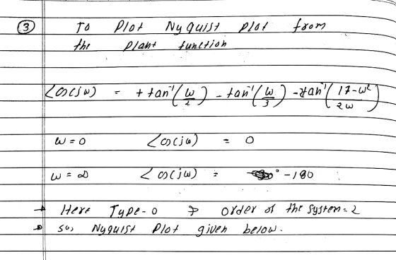
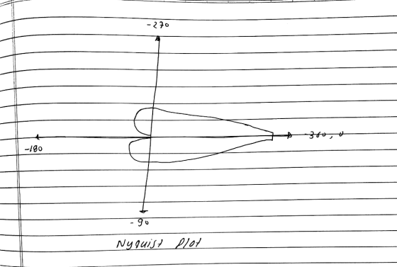
Consider the plant P(s) = (s3)(s22s + 17) in a feedback loop with a gain K...
Use rlocus in MATLAB to plot the root locus for a closed loop control system with the plant trans...
 Use rlocus in MATLAB to plot the root locus for a closed loop control system with the plant transfer function 8. z 2 2)2-0.1z +0.06 For what value of k is the closed loop system stable? 9. The characteristic equation for a control system is given as z2(0.2 +k)z 6k +2-0 Use Routh-Hurwitz criterion to find when the system is stable. 10. Use MATLAB to plot the root locus for the system given in Problem 9. Compare your conclusion in...
2. Given a unity feedback system with open-loop transfer function s+40s-I) a) For K-1, derive the...
 2. Given a unity feedback system with open-loop transfer function s+40s-I) a) For K-1, derive the expressions for the real and imaginary parts of G(jo). b) What happen to the real and imaginary parts of G(jo) for ω 0 and for Are there values of ω that either the real or imaginary part goes to zero? If not, compute Gijo) for some ovalue, say,, or 2, to help you sketch the Polar plot of Gja). c) d) Use Matlab to...
Problem 3: Consider a unity feedback system with a plant model given by 10(s- 5) and a controller...
 Problem 3: Consider a unity feedback system with a plant model given by 10(s- 5) and a controller given by s + p for K 0 and some real z and p. a) Use the root-locus technique to determine the sign of z and p so that the closed-loop system is stable for all K E (0, K) for some Ku> 0. b) Sketch the possible forms of the root-locus in terms of the pole and zero locations of Ge(s)....
Problem 3: (30) Consider the following systen where K is a proportional gain (K>0). s-2 (a) Sketch the root locus us...
 Problem 3: (30) Consider the following systen where K is a proportional gain (K>0). s-2 (a) Sketch the root locus using the below procedures. (1) find poles and zeros and locate on complex domain (2) find number of branches (3) find asymptotes including centroid and angles of asymptotes (4) intersection at imaginary axis (5) find the angle of departure (6) draw the root migration (b) Find the range of K for which the feedback system is asymptotically stable.
Problem 3:...
Problem 3: (30) Consider the following systen where K is a proportional gain (K>0). s-2 (a) Sketch the root locus using the below procedures. (1) find poles and zeros and locate on complex domain (2) find number of branches (3) find asymptotes including centroid and angles of asymptotes (4) intersection at imaginary axis (5) find the angle of departure (6) draw the root migration (b) Find the range of K for which the feedback system is asymptotically stable.
Problem 3:...
Problem 5: Suppose that you are to design a unity gain feedback controller for a first order plant. The plant...
 Problem 5: Suppose that you are to design a unity gain feedback controller for a first order plant. The plant and controller respectively take the form ,s+ p where K> 0, p. z are parameters to be specified. (a) Using root-locus methods, specify some p and z for which it is possible to make the closed-loop system strictly stable. Include a sketch of the closed-loop root locus, as well as the corresponding range of gains K for which the system...
Problem 2: For a unity feedback system where the plant is defined as G(s) K s(s+3)(s...
 Problem 2: For a unity feedback system where the plant is defined as G(s) K s(s+3)(s +5) a. Sketch the Nyquist Counter path and Nyquist diagram. Clearly show the real and imag- inary axis intercept points and the low and high frequency asymptotes. (10 pts) b. Using the Nyquist criterion, obtain the range of K in which the system can be stable, unstable, and also find the value of gain K for marginal stability. (7 pts) c. Calculate the frequency...
For the unity feedback system in the below figure, 1. EGO) R(s)) C(s) G(s)K (s 1) (s + 4) a) Sket...
 For the unity feedback system in the below figure, 1. EGO) R(s)) C(s) G(s)K (s 1) (s + 4) a) Sketch the bode plot with Matlab command bode0 b) Plot the nyquist diagram using Matlab command nyquist(0, find the system stability c) Find phase margin, gain margin, and crossover frequencies using Matlab command margin(0 and find the system stability
For the unity feedback system in the below figure, 1. EGO) R(s)) C(s) G(s)K (s 1) (s + 4) a) Sketch...
For the unity feedback system in the below figure, 1. EGO) R(s)) C(s) G(s)K (s 1) (s + 4) a) Sketch the bode plot with Matlab command bode0 b) Plot the nyquist diagram using Matlab command nyquist(0, find the system stability c) Find phase margin, gain margin, and crossover frequencies using Matlab command margin(0 and find the system stability
For the unity feedback system in the below figure, 1. EGO) R(s)) C(s) G(s)K (s 1) (s + 4) a) Sketch...
The characteristic equation (denominator of the closed-loop transfer function set equal to zero) is given s3 + 2s2 + (20K +7)s+ 100K Sketch the root locus of the given system above with respect to...
 The characteristic equation (denominator of the closed-loop transfer function set equal to zero) is given s3 + 2s2 + (20K +7)s+ 100K Sketch the root locus of the given system above with respect to K. [ Find the asymptotes and their angles, the break-away or break-in points, the angle of arrival or departure for the complex poles and zeros, imaginary axis crossing points, respectively (if any).
The characteristic equation (denominator of the closed-loop transfer function set equal to zero) is...
The characteristic equation (denominator of the closed-loop transfer function set equal to zero) is given s3 + 2s2 + (20K +7)s+ 100K Sketch the root locus of the given system above with respect to K. [ Find the asymptotes and their angles, the break-away or break-in points, the angle of arrival or departure for the complex poles and zeros, imaginary axis crossing points, respectively (if any).
The characteristic equation (denominator of the closed-loop transfer function set equal to zero) is...
Consider the following controller in a unity feedback configuration: (s + 10) C(s) = k· (s...
 Consider the following controller in a unity feedback configuration: (s + 10) C(s) = k· (s + 5) (a) (by hand) Using an approximation for the plant P(s) a 11 S +2)(s2 + 5s + 25) determine the proper L(s) and sketch an accurate Root Locus plot (b) (by hand) Once you have established the Root Locus, determine the range of k values that guarantees closed-loop stability using the L(jw) method along with the Root Locus plot.
Please solve part b and c and d !! Consider the closed loop system shown in...
 Please solve part b and c and d !!
Consider the closed loop system shown in Figure 4. The root locus of that system is shown in Figure 5 (s+40s+8) R(s) Y(s) Figure 4 System block diagram of Problem 4 a) On the root locus plot, sketch the region of possible roots of the dominant closed-loop poles such that the system response to a unit step has the following time domain specifications. [5] i. Damping ratio, 20.76 ii. Natural frequency,....
Please solve part b and c and d !!
Consider the closed loop system shown in Figure 4. The root locus of that system is shown in Figure 5 (s+40s+8) R(s) Y(s) Figure 4 System block diagram of Problem 4 a) On the root locus plot, sketch the region of possible roots of the dominant closed-loop poles such that the system response to a unit step has the following time domain specifications. [5] i. Damping ratio, 20.76 ii. Natural frequency,....
 Use rlocus in MATLAB to plot the root locus for a closed loop control system with the plant transfer function 8. z 2 2)2-0.1z +0.06 For what value of k is the closed loop system stable? 9. The characteristic equation for a control system is given as z2(0.2 +k)z 6k +2-0 Use Routh-Hurwitz criterion to find when the system is stable. 10. Use MATLAB to plot the root locus for the system given in Problem 9. Compare your conclusion in...
 2. Given a unity feedback system with open-loop transfer function s+40s-I) a) For K-1, derive the expressions for the real and imaginary parts of G(jo). b) What happen to the real and imaginary parts of G(jo) for ω 0 and for Are there values of ω that either the real or imaginary part goes to zero? If not, compute Gijo) for some ovalue, say,, or 2, to help you sketch the Polar plot of Gja). c) d) Use Matlab to...
 Problem 3: Consider a unity feedback system with a plant model given by 10(s- 5) and a controller given by s + p for K 0 and some real z and p. a) Use the root-locus technique to determine the sign of z and p so that the closed-loop system is stable for all K E (0, K) for some Ku> 0. b) Sketch the possible forms of the root-locus in terms of the pole and zero locations of Ge(s)....
 Problem 3: (30) Consider the following systen where K is a proportional gain (K>0). s-2 (a) Sketch the root locus using the below procedures. (1) find poles and zeros and locate on complex domain (2) find number of branches (3) find asymptotes including centroid and angles of asymptotes (4) intersection at imaginary axis (5) find the angle of departure (6) draw the root migration (b) Find the range of K for which the feedback system is asymptotically stable.
Problem 3:...
Problem 3: (30) Consider the following systen where K is a proportional gain (K>0). s-2 (a) Sketch the root locus using the below procedures. (1) find poles and zeros and locate on complex domain (2) find number of branches (3) find asymptotes including centroid and angles of asymptotes (4) intersection at imaginary axis (5) find the angle of departure (6) draw the root migration (b) Find the range of K for which the feedback system is asymptotically stable.
Problem 3:...
 Problem 5: Suppose that you are to design a unity gain feedback controller for a first order plant. The plant and controller respectively take the form ,s+ p where K> 0, p. z are parameters to be specified. (a) Using root-locus methods, specify some p and z for which it is possible to make the closed-loop system strictly stable. Include a sketch of the closed-loop root locus, as well as the corresponding range of gains K for which the system...
 Problem 2: For a unity feedback system where the plant is defined as G(s) K s(s+3)(s +5) a. Sketch the Nyquist Counter path and Nyquist diagram. Clearly show the real and imag- inary axis intercept points and the low and high frequency asymptotes. (10 pts) b. Using the Nyquist criterion, obtain the range of K in which the system can be stable, unstable, and also find the value of gain K for marginal stability. (7 pts) c. Calculate the frequency...
 For the unity feedback system in the below figure, 1. EGO) R(s)) C(s) G(s)K (s 1) (s + 4) a) Sketch the bode plot with Matlab command bode0 b) Plot the nyquist diagram using Matlab command nyquist(0, find the system stability c) Find phase margin, gain margin, and crossover frequencies using Matlab command margin(0 and find the system stability
For the unity feedback system in the below figure, 1. EGO) R(s)) C(s) G(s)K (s 1) (s + 4) a) Sketch...
For the unity feedback system in the below figure, 1. EGO) R(s)) C(s) G(s)K (s 1) (s + 4) a) Sketch the bode plot with Matlab command bode0 b) Plot the nyquist diagram using Matlab command nyquist(0, find the system stability c) Find phase margin, gain margin, and crossover frequencies using Matlab command margin(0 and find the system stability
For the unity feedback system in the below figure, 1. EGO) R(s)) C(s) G(s)K (s 1) (s + 4) a) Sketch...
 The characteristic equation (denominator of the closed-loop transfer function set equal to zero) is given s3 + 2s2 + (20K +7)s+ 100K Sketch the root locus of the given system above with respect to K. [ Find the asymptotes and their angles, the break-away or break-in points, the angle of arrival or departure for the complex poles and zeros, imaginary axis crossing points, respectively (if any).
The characteristic equation (denominator of the closed-loop transfer function set equal to zero) is...
The characteristic equation (denominator of the closed-loop transfer function set equal to zero) is given s3 + 2s2 + (20K +7)s+ 100K Sketch the root locus of the given system above with respect to K. [ Find the asymptotes and their angles, the break-away or break-in points, the angle of arrival or departure for the complex poles and zeros, imaginary axis crossing points, respectively (if any).
The characteristic equation (denominator of the closed-loop transfer function set equal to zero) is...
 Consider the following controller in a unity feedback configuration: (s + 10) C(s) = k· (s + 5) (a) (by hand) Using an approximation for the plant P(s) a 11 S +2)(s2 + 5s + 25) determine the proper L(s) and sketch an accurate Root Locus plot (b) (by hand) Once you have established the Root Locus, determine the range of k values that guarantees closed-loop stability using the L(jw) method along with the Root Locus plot.
 Please solve part b and c and d !!
Consider the closed loop system shown in Figure 4. The root locus of that system is shown in Figure 5 (s+40s+8) R(s) Y(s) Figure 4 System block diagram of Problem 4 a) On the root locus plot, sketch the region of possible roots of the dominant closed-loop poles such that the system response to a unit step has the following time domain specifications. [5] i. Damping ratio, 20.76 ii. Natural frequency,....
Please solve part b and c and d !!
Consider the closed loop system shown in Figure 4. The root locus of that system is shown in Figure 5 (s+40s+8) R(s) Y(s) Figure 4 System block diagram of Problem 4 a) On the root locus plot, sketch the region of possible roots of the dominant closed-loop poles such that the system response to a unit step has the following time domain specifications. [5] i. Damping ratio, 20.76 ii. Natural frequency,....
Most questions answered within 3 hours.
-
a) Find the pressure difference on an airplane wing if air flows
over the upper surface...
asked 4 seconds ago -
Write an assessment of the current business analysis of Hilton
Worldwide using Porters 5 Forces analysis.
asked 10 minutes ago -
i need help on this
Chapter 9 Section 3 Question 1:
Rudy puts this poster, with...
asked 19 minutes ago -
True or false Assembly x86
41. _____ The program counter is a pointer to the
instruction....
asked 19 minutes ago -
You have conducted an experiment to try to demonstrate that
growth factor receptor X protein (GFRX)...
asked 35 minutes ago -
The Gross Profit ratio for 2014 is 57.07%
Assume that Campbell's net sales for the first...
asked 34 minutes ago -
Thoroughly discuss the various current and proposed solutions to
anthropogenic influences resulting in Global Climate Change....
asked 39 minutes ago -
BLOG EXERCISE: You are writing a weekly intranet blog for the
CEO of a large Canadian...
asked 42 minutes ago -
calculate ΔGrxn at 36 ∘C. N2O4(g)→2NO2(g)
asked 42 minutes ago -
Present and Future Values of Single Cash Flows for Different
Periods
Find the following values, using...
asked 45 minutes ago -
Which types of mutations in DNA can lead to the translation of a
non-functional protein product?...
asked 44 minutes ago -
Many structures are composed of individual elements that react
in unison when forces are applied. the...
asked 45 minutes ago