
Homework Answers

To find and plot the Pole Zero Map
The zeros are at locations where the numerator polynomial is zero. So

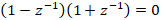
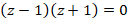

So the zeros are at

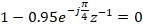
The poles are at locations where the denominator polynomial is zero. So

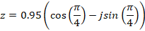
First Pole
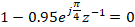


Another way to find the pole is

So the pole is at

The pole is at the point at an angle
 at a distance
0.95.
at a distance
0.95.
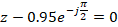
Second Pole


Another way to find the pole is

So the pole is at

The pole is at the point at an angle
 at a distance
0.95.
at a distance
0.95.
Third Pole


Another way to find the pole is

So the pole is at

The pole is at the point at an angle
 at a distance
0.95.
at a distance
0.95.
Fourth Pole


Another way to find the pole is

So the pole is at

The pole is at the point at an angle
 at a distance
0.95.
at a distance
0.95.
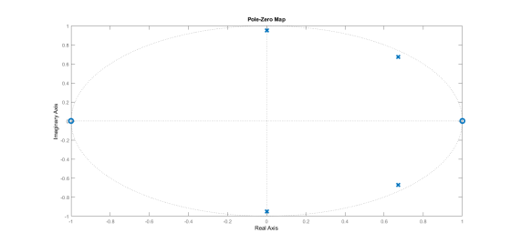
So the poles are at

Hence the pole zero plot will be
To find and plot the Magnitude Response

We know that


So
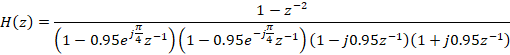

Using

We get


To get the frequency response put


Using MATLAB
clc;
clear all;
close all;
b = [1, 0, -1];
a1 = [1, -1.3435, 0.9025];
a2 = [1, 0, 0.9025];
a = conv(a1, a2);
w = -pi:pi/1000:pi;
H = freqz(b, a, w);
plot(w/pi, abs(H), 'linewidth', 2);
grid;
xlabel('Normalized Frequency, \omega (\times \pi units)');
ylabel('|H(e^{j\omega})|');
title('Magnitude Response');
sys = tf(b,a,1)
figure
pzmap(sys)
After executing we get

Add Answer to:
please show steps and formulas.
Plot the magnitude of the and the pole- zero plot frequency...
2. Consider a second IIR filter a. Determine the system function H(z), pole-zero location (patterns), and plot the pole-zero pattern. b. Determine the analytical expression for frequency response...
 2. Consider a second IIR filter a. Determine the system function H(z), pole-zero location (patterns), and plot the pole-zero pattern. b. Determine the analytical expression for frequency response, magnitude, and phase response. c. Choose b so that the maximum magnitude response is equal to 1. d. Plot the pole-zero pattern and the magnitude of the frequency response as a function of normal frequency.
2. Consider a second IIR filter a. Determine the system function H(z), pole-zero location (patterns), and plot...
2. Consider a second IIR filter a. Determine the system function H(z), pole-zero location (patterns), and plot the pole-zero pattern. b. Determine the analytical expression for frequency response, magnitude, and phase response. c. Choose b so that the maximum magnitude response is equal to 1. d. Plot the pole-zero pattern and the magnitude of the frequency response as a function of normal frequency.
2. Consider a second IIR filter a. Determine the system function H(z), pole-zero location (patterns), and plot...
For each of the transfer functions given below, draw the pole-zero plot and plot the magnitude separate from the phase as a function of frequency. Show only the asymptotic terms that make up the tra...
 For each of the transfer functions given below, draw the pole-zero plot and plot the magnitude separate from the phase as a function of frequency. Show only the asymptotic terms that make up the transfer function and then add them to show the composite plot. You can verify your plots (to some extent) by using MATLAB to generate the plots but only as a check that the work you have done is correct. The work that will count for points...
5) Design a one-pole, one-zero passive filter to have a low-frequency gain of -32 dB, a high-freq...
 please show all steps and matlab plot ,
5) Design a one-pole, one-zero passive filter to have a low-frequency gain of -32 dB, a high-frequency gain of 0 dB, and a cutoff frequency of 2,000 Hz. Specify the circuit and all component values. Use Matlab to plot the magnitude and phase frequency response for your filter.
5) Design a one-pole, one-zero passive filter to have a low-frequency gain of -32 dB, a high-frequency gain of 0 dB, and a cutoff...
please show all steps and matlab plot ,
5) Design a one-pole, one-zero passive filter to have a low-frequency gain of -32 dB, a high-frequency gain of 0 dB, and a cutoff frequency of 2,000 Hz. Specify the circuit and all component values. Use Matlab to plot the magnitude and phase frequency response for your filter.
5) Design a one-pole, one-zero passive filter to have a low-frequency gain of -32 dB, a high-frequency gain of 0 dB, and a cutoff...
I (K Pole-Zero Plot #1 Pole-Eero Plot 15 L. Pole-Zero Plot IMI 4z1 15 Prde-Zero Plot...
 I (K Pole-Zero Plot #1 Pole-Eero Plot 15 L. Pole-Zero Plot IMI 4z1 15 Prde-Zero Plot #5 Pole-Zero Plat #6 Tine Index (n) Problem P-10.20. Match a pole-zero plot (1-6) to each of the impulse response plots (J-N) shown above (Figure P-10.20 from p. 464) Note: Beach Board causes the magnitude Impulse Response Plot number order to be in random order Pole-Zero Plot #1 Pole-Zero Plot #2 Pole-Zero Plot #3 1, hin] Plot (N) hin] Plot (K) h[n] Plot (M)...
Below is the zero and poles plot of a system. What is the magnitude response of this system? Pole...
 Below is the zero and poles plot of a system. What is the magnitude response of this system? Pole/Zero Plot 0.5 0 0.5 0.5 0 Real Part 0.5 H(J) : (exp(2*90i*theta)-2"exp(%itthet exp(2-i.6)-2 exp(i-0)+2 exp(2 i.)-exp(i.0)+0.5 Your last answer was interpreted as follows: CHR The variables found in your answer were: [e] Incorrect answer.
Below is the zero and poles plot of a system. What is the magnitude response of this system? Pole/Zero Plot 0.5 0 0.5 0.5 0 Real Part...
Below is the zero and poles plot of a system. What is the magnitude response of this system? Pole/Zero Plot 0.5 0 0.5 0.5 0 Real Part 0.5 H(J) : (exp(2*90i*theta)-2"exp(%itthet exp(2-i.6)-2 exp(i-0)+2 exp(2 i.)-exp(i.0)+0.5 Your last answer was interpreted as follows: CHR The variables found in your answer were: [e] Incorrect answer.
Below is the zero and poles plot of a system. What is the magnitude response of this system? Pole/Zero Plot 0.5 0 0.5 0.5 0 Real Part...
no need for pole-zero plot 7. Determine the system function, magnitude response, and phase response of...
 no need for pole-zero plot
7. Determine the system function, magnitude response, and phase response of the fol- lowing systems and use the pole-zero pattern to explain the shape of their magnitude response (a) y[n] = 1(x(n]-x(n-1), ln -2
no need for pole-zero plot
7. Determine the system function, magnitude response, and phase response of the fol- lowing systems and use the pole-zero pattern to explain the shape of their magnitude response (a) y[n] = 1(x(n]-x(n-1), ln -2
For each of the transfer functions given below, draw the pole-zero plot and using the log- semilog paper provided on Blackboard to plot the magnitude separate from the phase as a function of frequenc...
 For each of the transfer functions given below, draw the pole-zero plot and using the log- semilog paper provided on Blackboard to plot the magnitude separate from the phase as a function of frequency. Show only the asymptotic terms that make up the transfer function and then add them to show the composite plot. You can verify your plots (to some extent) by using MATLAB to generate the plots but only as a check that the work you have done...
Problem 4 Questions about the frequency response of an FIR filter: (a) Determine a formula for th...
 Please show all work
Problem 4 Questions about the frequency response of an FIR filter: (a) Determine a formula for the frequency response of an FIR filter defined by the pole-zero plot below: Pole-Zero Plot #1 0.5 -0.5 -1 1 -0.5 0 051 Real part (b) For the FIR filter in part (a), write a simplified version of the frequency response H(e'ω) and use it to prove that the maximum value of the frequency response magnitude will be at ω-tr/2....
Please show all work
Problem 4 Questions about the frequency response of an FIR filter: (a) Determine a formula for the frequency response of an FIR filter defined by the pole-zero plot below: Pole-Zero Plot #1 0.5 -0.5 -1 1 -0.5 0 051 Real part (b) For the FIR filter in part (a), write a simplified version of the frequency response H(e'ω) and use it to prove that the maximum value of the frequency response magnitude will be at ω-tr/2....
The pole-zero plot of a cosine oscillator filter is shown below. The oscillation frequency is one...
 The pole-zero plot of a cosine oscillator filter is shown below. The oscillation frequency is one quarter of the sampling frequency (Fs/4). Pole-Zero Plot for the Non-Damped Cosine Oscillator zp R-1 0.8 06 0.4 0.2 zct zc2 2nd order -0.2 -0.4 -0.6 -0.8 -1 zp -1 -0.5 0.5 Real Part O True False Imaginary Part
Question 3 The pole-zero plot of a sinusoidal oscillator filter is shown below. If the system...
 Question 3 The pole-zero plot of a sinusoidal oscillator filter is shown below. If the system is working at Fs = 8000Hz, the output tone has a frequency of 1000 Hz. Pole-Zero Plot for the Non-Damped Cosine Oscillator Imaginary Part 201 202 2nd order The X zp -1 -0. 50 0. 51 Real Part True False
 2. Consider a second IIR filter a. Determine the system function H(z), pole-zero location (patterns), and plot the pole-zero pattern. b. Determine the analytical expression for frequency response, magnitude, and phase response. c. Choose b so that the maximum magnitude response is equal to 1. d. Plot the pole-zero pattern and the magnitude of the frequency response as a function of normal frequency.
2. Consider a second IIR filter a. Determine the system function H(z), pole-zero location (patterns), and plot...
2. Consider a second IIR filter a. Determine the system function H(z), pole-zero location (patterns), and plot the pole-zero pattern. b. Determine the analytical expression for frequency response, magnitude, and phase response. c. Choose b so that the maximum magnitude response is equal to 1. d. Plot the pole-zero pattern and the magnitude of the frequency response as a function of normal frequency.
2. Consider a second IIR filter a. Determine the system function H(z), pole-zero location (patterns), and plot...
 For each of the transfer functions given below, draw the pole-zero plot and plot the magnitude separate from the phase as a function of frequency. Show only the asymptotic terms that make up the transfer function and then add them to show the composite plot. You can verify your plots (to some extent) by using MATLAB to generate the plots but only as a check that the work you have done is correct. The work that will count for points...
 please show all steps and matlab plot ,
5) Design a one-pole, one-zero passive filter to have a low-frequency gain of -32 dB, a high-frequency gain of 0 dB, and a cutoff frequency of 2,000 Hz. Specify the circuit and all component values. Use Matlab to plot the magnitude and phase frequency response for your filter.
5) Design a one-pole, one-zero passive filter to have a low-frequency gain of -32 dB, a high-frequency gain of 0 dB, and a cutoff...
please show all steps and matlab plot ,
5) Design a one-pole, one-zero passive filter to have a low-frequency gain of -32 dB, a high-frequency gain of 0 dB, and a cutoff frequency of 2,000 Hz. Specify the circuit and all component values. Use Matlab to plot the magnitude and phase frequency response for your filter.
5) Design a one-pole, one-zero passive filter to have a low-frequency gain of -32 dB, a high-frequency gain of 0 dB, and a cutoff...
 I (K Pole-Zero Plot #1 Pole-Eero Plot 15 L. Pole-Zero Plot IMI 4z1 15 Prde-Zero Plot #5 Pole-Zero Plat #6 Tine Index (n) Problem P-10.20. Match a pole-zero plot (1-6) to each of the impulse response plots (J-N) shown above (Figure P-10.20 from p. 464) Note: Beach Board causes the magnitude Impulse Response Plot number order to be in random order Pole-Zero Plot #1 Pole-Zero Plot #2 Pole-Zero Plot #3 1, hin] Plot (N) hin] Plot (K) h[n] Plot (M)...
 Below is the zero and poles plot of a system. What is the magnitude response of this system? Pole/Zero Plot 0.5 0 0.5 0.5 0 Real Part 0.5 H(J) : (exp(2*90i*theta)-2"exp(%itthet exp(2-i.6)-2 exp(i-0)+2 exp(2 i.)-exp(i.0)+0.5 Your last answer was interpreted as follows: CHR The variables found in your answer were: [e] Incorrect answer.
Below is the zero and poles plot of a system. What is the magnitude response of this system? Pole/Zero Plot 0.5 0 0.5 0.5 0 Real Part...
Below is the zero and poles plot of a system. What is the magnitude response of this system? Pole/Zero Plot 0.5 0 0.5 0.5 0 Real Part 0.5 H(J) : (exp(2*90i*theta)-2"exp(%itthet exp(2-i.6)-2 exp(i-0)+2 exp(2 i.)-exp(i.0)+0.5 Your last answer was interpreted as follows: CHR The variables found in your answer were: [e] Incorrect answer.
Below is the zero and poles plot of a system. What is the magnitude response of this system? Pole/Zero Plot 0.5 0 0.5 0.5 0 Real Part...
 no need for pole-zero plot
7. Determine the system function, magnitude response, and phase response of the fol- lowing systems and use the pole-zero pattern to explain the shape of their magnitude response (a) y[n] = 1(x(n]-x(n-1), ln -2
no need for pole-zero plot
7. Determine the system function, magnitude response, and phase response of the fol- lowing systems and use the pole-zero pattern to explain the shape of their magnitude response (a) y[n] = 1(x(n]-x(n-1), ln -2
 For each of the transfer functions given below, draw the pole-zero plot and using the log- semilog paper provided on Blackboard to plot the magnitude separate from the phase as a function of frequency. Show only the asymptotic terms that make up the transfer function and then add them to show the composite plot. You can verify your plots (to some extent) by using MATLAB to generate the plots but only as a check that the work you have done...
 Please show all work
Problem 4 Questions about the frequency response of an FIR filter: (a) Determine a formula for the frequency response of an FIR filter defined by the pole-zero plot below: Pole-Zero Plot #1 0.5 -0.5 -1 1 -0.5 0 051 Real part (b) For the FIR filter in part (a), write a simplified version of the frequency response H(e'ω) and use it to prove that the maximum value of the frequency response magnitude will be at ω-tr/2....
Please show all work
Problem 4 Questions about the frequency response of an FIR filter: (a) Determine a formula for the frequency response of an FIR filter defined by the pole-zero plot below: Pole-Zero Plot #1 0.5 -0.5 -1 1 -0.5 0 051 Real part (b) For the FIR filter in part (a), write a simplified version of the frequency response H(e'ω) and use it to prove that the maximum value of the frequency response magnitude will be at ω-tr/2....
 The pole-zero plot of a cosine oscillator filter is shown below. The oscillation frequency is one quarter of the sampling frequency (Fs/4). Pole-Zero Plot for the Non-Damped Cosine Oscillator zp R-1 0.8 06 0.4 0.2 zct zc2 2nd order -0.2 -0.4 -0.6 -0.8 -1 zp -1 -0.5 0.5 Real Part O True False Imaginary Part
 Question 3 The pole-zero plot of a sinusoidal oscillator filter is shown below. If the system is working at Fs = 8000Hz, the output tone has a frequency of 1000 Hz. Pole-Zero Plot for the Non-Damped Cosine Oscillator Imaginary Part 201 202 2nd order The X zp -1 -0. 50 0. 51 Real Part True False
Most questions answered within 3 hours.
-
1) If Nominal GDP is $16,000 billion and the GDP deflator is 50,
then Real GDP...
asked 1 minute from now -
D. A student completed 20 courses in the School of Arts and
Sciences. Her grades in...
asked 1 hour ago -
teo
pucks moving on a frictionless air table are about to collide. the
1.5 kg puck...
asked 1 hour ago -
Problem #1
The area between Z = 0 and Z = 2.50
The area between Z...
asked 3 hours ago -
1. What is the meaning of the term communication style?
2. What are the benefits to...
asked 2 hours ago -
9.) You are buying a car that cost $26,500. You make payments of
$412 each month...
asked 3 hours ago -
. Suppose a discrete random variable has probability
distribution
P(x) = .2 if x = 0...
asked 4 hours ago -
Under the influence of its drive force, a snowmobile is moving
at a constant velocity along...
asked 4 hours ago -
Why do organizations decline? What steps can top
management take to halt, decline, and restore organizational...
asked 4 hours ago -
What mechanisms Drive speciation??
(I.e. what was Dawins theory on the orgin of species, and how...
asked 6 hours ago -
The manager at a car assembly plant believes that the mean
assembly time for a car...
asked 7 hours ago -
Which of the following is true of electron capture?
A) It decreases the nuclide's mass number...
asked 8 hours ago