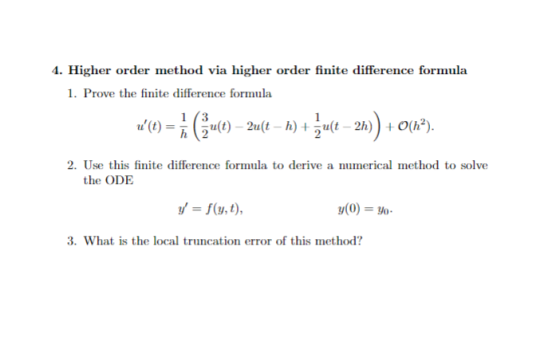
4. Higher order method via higher order finite difference formula
Homework Answers


Add Answer to:
4. Higher order method via higher order finite difference
formula
4. Higher order method via higher...
Question 1 15 Points) It is always desirable to have/ use the finite difference approximation wit...
 Question 1 15 Points) It is always desirable to have/ use the finite difference approximation with error term. Please using the Taylor Series: higher order of truncation sw(x) h" +R 2! 3! (I) Derive the following forward difference approximation of the 2nd orde 2) What is the order of error for this case? derivative of f(x). f" derivative off(x) h2
Question 1 15 Points) It is always desirable to have/ use the finite difference approximation with error term. Please using...
Question 1 15 Points) It is always desirable to have/ use the finite difference approximation with error term. Please using the Taylor Series: higher order of truncation sw(x) h" +R 2! 3! (I) Derive the following forward difference approximation of the 2nd orde 2) What is the order of error for this case? derivative of f(x). f" derivative off(x) h2
Question 1 15 Points) It is always desirable to have/ use the finite difference approximation with error term. Please using...
5. Following an approach similar to what was performed in lecture for the first forward finite-divided-difference...
 5. Following an approach similar to what was performed in lecture for the first forward finite-divided-difference equation with local truncation error Oſhº), please derive the following expression for the first backward finite-divided-difference equation with location truncation error O(h?). f'(x) – 3 f(xi) – 4 f(xi-1) + f(xi-2) 2 h
(b) Derive a numerical differentiation formula of order O(h4) by applying Richardson ertrapolation to 2 MI...
 (b) Derive a numerical differentiation formula of order O(h4) by applying Richardson ertrapolation to 2 MI 2h 120 Richardson extrapolation is a useful way to obtain higher precision from either an approximate formula or a code, provided you know precisely what the truncation error of the approximation is. The truncation error is of order h2 above. So what we will do is use the above formula over rth/2 to derive another approximation for the first derivative. The add/subtract these two...
1. U se Taylors formula to derive the forward, backward and center difference for- mulas for the derivative /"(x) a...
 1. U se Taylors formula to derive the forward, backward and center difference for- mulas for the derivative /"(x) at a point x Use the reminder in Taylors formula to determine the order (truncation error) of the numerical approximation of the derivative in each case.
1. U se Taylors formula to derive the forward, backward and center difference for- mulas for the derivative /"(x) at a point x Use the reminder in Taylors formula to determine the order (truncation error)...
1. U se Taylors formula to derive the forward, backward and center difference for- mulas for the derivative /"(x) at a point x Use the reminder in Taylors formula to determine the order (truncation error) of the numerical approximation of the derivative in each case.
1. U se Taylors formula to derive the forward, backward and center difference for- mulas for the derivative /"(x) at a point x Use the reminder in Taylors formula to determine the order (truncation error)...
ASAP PLEASE e) Explain the idea of the Gauss integration formula. f Show on a figure the local and global truncation error for the first two iterations of a ODE solver g) Solve graphically the ODE h)...
 ASAP PLEASE
e) Explain the idea of the Gauss integration formula. f Show on a figure the local and global truncation error for the first two iterations of a ODE solver g) Solve graphically the ODE h) Explain how numerical adaptive ODE solvers works i) When is a numerical method for solving differential equations considered to be dy dx unstable ? Which parameter(s) is (are) influencing this stability (or instability)? j In general the total error done by any numerical...
ASAP PLEASE
e) Explain the idea of the Gauss integration formula. f Show on a figure the local and global truncation error for the first two iterations of a ODE solver g) Solve graphically the ODE h) Explain how numerical adaptive ODE solvers works i) When is a numerical method for solving differential equations considered to be dy dx unstable ? Which parameter(s) is (are) influencing this stability (or instability)? j In general the total error done by any numerical...
Find the truncation error and the order of accuracy of the following finite difference representation. dx2 (Ax)2 F...
 Find the truncation error and the order of accuracy of the following finite difference representation. dx2 (Ax)2
Find the truncation error and the order of accuracy of the following finite difference representation. dx2 (Ax)2
Find the truncation error and the order of accuracy of the following finite difference representation. dx2 (Ax)2
For the following set of data, calculate the derivative using the higher order finite-difference approximations for...
 For the following set of data, calculate the derivative using the higher order finite-difference approximations for each data point, as shown in Figures 21.43-21.5. Round your answers to 2 decimal places, if needed. 0 0.5 1.0 1.5 2.0 2.5 X f(x) 33 72 80 10 25 58 Using the forward finite-difference approximation: f'(0) ~ f'(0.5) Using the centered finite-difference approximation: f'(1.0) f'(1.5) Using the backward finite-difference approximation: f'(2.0) f'(2.5) 은 8
4. (25 points) Solve the following ODE using classical 4th-order Runge- Kutta method within the domain...
 4. (25 points) Solve the following ODE using classical 4th-order Runge- Kutta method within the domain of x = 0 to x= 2 with step size h = 1: dy 3 dr=y+ 6x3 dx The initial condition is y(0) = 1. If the analytical solution of the ODE is y = 21.97x - 5.15; calculate the error between true solution and numerical solution at y(1) and y(2).
this is numerical analysis. Please do a and b 4. Consider the ordinary differential equation 1'(x)...
 this is numerical analysis. Please do a and b
4. Consider the ordinary differential equation 1'(x) = f(x, y(x)), y(ro) = Yo. (1) (a) Use numerical integration to derive the trapezoidal method for the above with uniform step size h. (You don't have to give the truncation error.) (b) Given below is a multistep method for solving (1) (with uniform step size h): bo +1 = 34 – 2n=1 + h (362. Yn) = f(n=1, 4n-1)) What is the truncation...
this is numerical analysis. Please do a and b
4. Consider the ordinary differential equation 1'(x) = f(x, y(x)), y(ro) = Yo. (1) (a) Use numerical integration to derive the trapezoidal method for the above with uniform step size h. (You don't have to give the truncation error.) (b) Given below is a multistep method for solving (1) (with uniform step size h): bo +1 = 34 – 2n=1 + h (362. Yn) = f(n=1, 4n-1)) What is the truncation...
Problem #3: The Ralston method is a second-order method that can be used to solve an...
 Problem #3: The Ralston method is a second-order method that can be used to solve an initial-value, first-order ordinary differential equation. The algorithm is given below: 2 Yi+1 = yi + k +k2)h Where kı = f(ti,y;) 3 k2 = ft;+ -h, y; +-kih You are asked to do the following: 3.1 Following that given in Inclass activity #10a, develop a MATLAB function to implement the algorithm for any given function, the time span, and the initial value. 3.2 Use...
 Question 1 15 Points) It is always desirable to have/ use the finite difference approximation with error term. Please using the Taylor Series: higher order of truncation sw(x) h" +R 2! 3! (I) Derive the following forward difference approximation of the 2nd orde 2) What is the order of error for this case? derivative of f(x). f" derivative off(x) h2
Question 1 15 Points) It is always desirable to have/ use the finite difference approximation with error term. Please using...
Question 1 15 Points) It is always desirable to have/ use the finite difference approximation with error term. Please using the Taylor Series: higher order of truncation sw(x) h" +R 2! 3! (I) Derive the following forward difference approximation of the 2nd orde 2) What is the order of error for this case? derivative of f(x). f" derivative off(x) h2
Question 1 15 Points) It is always desirable to have/ use the finite difference approximation with error term. Please using...
 5. Following an approach similar to what was performed in lecture for the first forward finite-divided-difference equation with local truncation error Oſhº), please derive the following expression for the first backward finite-divided-difference equation with location truncation error O(h?). f'(x) – 3 f(xi) – 4 f(xi-1) + f(xi-2) 2 h
 (b) Derive a numerical differentiation formula of order O(h4) by applying Richardson ertrapolation to 2 MI 2h 120 Richardson extrapolation is a useful way to obtain higher precision from either an approximate formula or a code, provided you know precisely what the truncation error of the approximation is. The truncation error is of order h2 above. So what we will do is use the above formula over rth/2 to derive another approximation for the first derivative. The add/subtract these two...
 1. U se Taylors formula to derive the forward, backward and center difference for- mulas for the derivative /"(x) at a point x Use the reminder in Taylors formula to determine the order (truncation error) of the numerical approximation of the derivative in each case.
1. U se Taylors formula to derive the forward, backward and center difference for- mulas for the derivative /"(x) at a point x Use the reminder in Taylors formula to determine the order (truncation error)...
1. U se Taylors formula to derive the forward, backward and center difference for- mulas for the derivative /"(x) at a point x Use the reminder in Taylors formula to determine the order (truncation error) of the numerical approximation of the derivative in each case.
1. U se Taylors formula to derive the forward, backward and center difference for- mulas for the derivative /"(x) at a point x Use the reminder in Taylors formula to determine the order (truncation error)...
 ASAP PLEASE
e) Explain the idea of the Gauss integration formula. f Show on a figure the local and global truncation error for the first two iterations of a ODE solver g) Solve graphically the ODE h) Explain how numerical adaptive ODE solvers works i) When is a numerical method for solving differential equations considered to be dy dx unstable ? Which parameter(s) is (are) influencing this stability (or instability)? j In general the total error done by any numerical...
ASAP PLEASE
e) Explain the idea of the Gauss integration formula. f Show on a figure the local and global truncation error for the first two iterations of a ODE solver g) Solve graphically the ODE h) Explain how numerical adaptive ODE solvers works i) When is a numerical method for solving differential equations considered to be dy dx unstable ? Which parameter(s) is (are) influencing this stability (or instability)? j In general the total error done by any numerical...
 Find the truncation error and the order of accuracy of the following finite difference representation. dx2 (Ax)2
Find the truncation error and the order of accuracy of the following finite difference representation. dx2 (Ax)2
Find the truncation error and the order of accuracy of the following finite difference representation. dx2 (Ax)2
 For the following set of data, calculate the derivative using the higher order finite-difference approximations for each data point, as shown in Figures 21.43-21.5. Round your answers to 2 decimal places, if needed. 0 0.5 1.0 1.5 2.0 2.5 X f(x) 33 72 80 10 25 58 Using the forward finite-difference approximation: f'(0) ~ f'(0.5) Using the centered finite-difference approximation: f'(1.0) f'(1.5) Using the backward finite-difference approximation: f'(2.0) f'(2.5) 은 8
 4. (25 points) Solve the following ODE using classical 4th-order Runge- Kutta method within the domain of x = 0 to x= 2 with step size h = 1: dy 3 dr=y+ 6x3 dx The initial condition is y(0) = 1. If the analytical solution of the ODE is y = 21.97x - 5.15; calculate the error between true solution and numerical solution at y(1) and y(2).
 this is numerical analysis. Please do a and b
4. Consider the ordinary differential equation 1'(x) = f(x, y(x)), y(ro) = Yo. (1) (a) Use numerical integration to derive the trapezoidal method for the above with uniform step size h. (You don't have to give the truncation error.) (b) Given below is a multistep method for solving (1) (with uniform step size h): bo +1 = 34 – 2n=1 + h (362. Yn) = f(n=1, 4n-1)) What is the truncation...
this is numerical analysis. Please do a and b
4. Consider the ordinary differential equation 1'(x) = f(x, y(x)), y(ro) = Yo. (1) (a) Use numerical integration to derive the trapezoidal method for the above with uniform step size h. (You don't have to give the truncation error.) (b) Given below is a multistep method for solving (1) (with uniform step size h): bo +1 = 34 – 2n=1 + h (362. Yn) = f(n=1, 4n-1)) What is the truncation...
 Problem #3: The Ralston method is a second-order method that can be used to solve an initial-value, first-order ordinary differential equation. The algorithm is given below: 2 Yi+1 = yi + k +k2)h Where kı = f(ti,y;) 3 k2 = ft;+ -h, y; +-kih You are asked to do the following: 3.1 Following that given in Inclass activity #10a, develop a MATLAB function to implement the algorithm for any given function, the time span, and the initial value. 3.2 Use...
Most questions answered within 3 hours.
-
A bowling ball (solid sphere) of mass 5.0 kg and
radius of 11cm. What is theangular...
asked 3 minutes ago -
Assume you used Analysis of Variance to compare the student debt
for 100 college graduates--25 from...
asked 7 minutes ago -
jane 49 contributed 6000 to her ira on November 11
2018 she comes into your office...
asked 3 minutes ago -
a company just paid an annual dividend of $1.20 per share. the
share is priced at...
asked 6 minutes ago -
What was happening in the workplace before the signing of the
Civil Rights Act of 1964?
asked 10 minutes ago -
The probability that a randomly selected teenager studied at
least once during a week was only...
asked 15 minutes ago -
At 20.0°C, the vapor pressure of ethanol is 45.0 torr, and the
vapor pressure of methanol...
asked 17 minutes ago -
13.
Given the following definitions:
U = {1, 2, 3, 4, 5, 6, 7}
A =...
asked 25 minutes ago -
1. Let us again continue with analyses of data from the study of
M Daviglus et...
asked 26 minutes ago -
Consider the following data for a dependent variable y and two
independent variables, x1 and x2....
asked 25 minutes ago -
Research paper on a Sex Crime and Policy Topic
Including all 3 origins “sex crime and...
asked 27 minutes ago -
6. What volume will 40.0mL of nitrogen, measured at 15.0°C and
780.0torr, occupy at STP?
7....
asked 27 minutes ago