Question

6. Deriving the short-run supply curve Consider the competitive market for halogen lamps. The following graph shows the marginal cost (MC), average total cost (ATC), and average variable cost (AVC) curves for a typical firm in the industry. 90 80 6 2 50 3 40 30 AVC 10 20 30 40 50 70 100 QUANTITY Thousands of lamps)

Answer 1

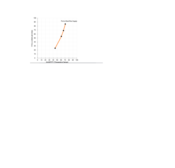
Following is the complete table -

Price	Quantity	Produce or Shut down	Profit or Loss
15	0	Shut down	Loss
20	0	Shut down	Loss
25	Either 0 or 45,000	Either	Loss
55	60,000	Produce	Break-even
70	65,000	Produce	Profit
85	70,000	Produce	Profit

Following is the firm's short-run supply schedule -

Price	Quantity
25	45,000
55	60,000
70	65,000
85	70,000

Following is the firm's short-run supply curve -

100 90 80 70 80 50 40 30 20 10 Firms Short-Run Supply 0 10 20 30 40 50 60 70 80 90 100

There are 5 firms in this industry.

Following is the industry's short-run supply schedule -

Price	Individual Supply	Industry Supply
25	45,000	45,000 * 5 = 225,000
55	60,000	60,000 * 5 = 300,000
70	65,000	65,000 * 5 = 325,000
85	70,000	70,000 * 5 = 350,000

Following is the industry's short-run supply curve -

100 00Demand 90 80 70 60 50 Industry's Short-Run Supply Equilibrium 30 20 10 0 50 100 150 200 250 300 350 400 450 500 QUANTITY (Thousands of lamps)

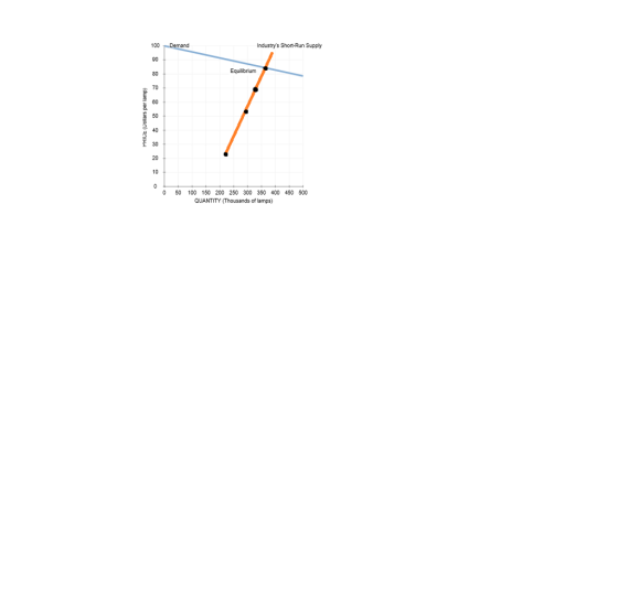
At the current short-run market price, firm will earn economic profit in the short-run. In the long-run, there will be entry of new firms in the industry.