![2. Given the unity feedback system with K(s +4) G(s) find the following: a) The range of K that keeps the system stable. 120]](http://img.homeworklib.com/questions/5b089cf0-c7d8-11eb-aa82-7fb6cc4f848c.png?x-oss-process=image/resize,w_560)
Homework Answers


Add Answer to:
2. Given the unity feedback system with K(s +4) G(s) find the following: a) The range...
Given the unity feedback system of Figure 1, find the following The range of K that keeps the system stable The v...
 Given the unity feedback system of Figure 1, find the following The range of K that keeps the system stable The value of K that makes the system oscillate The frequency of oscillation when K is set to the value that makes the system oscillate with: K(s-1)(s-2) (s+2)(s2+2s + 2) G(s) C(s) R(s) E(s) + G(s) Figure: 1
Given the unity feedback system of Figure 1, find the following The range of K that keeps the system stable The value...
Given the unity feedback system of Figure 1, find the following The range of K that keeps the system stable The value of K that makes the system oscillate The frequency of oscillation when K is set to the value that makes the system oscillate with: K(s-1)(s-2) (s+2)(s2+2s + 2) G(s) C(s) R(s) E(s) + G(s) Figure: 1
Given the unity feedback system of Figure 1, find the following The range of K that keeps the system stable The value...
Puge 328 polf prt 33 Question 3 [20 Marks (a) K(s+4) $(s+1)(s+2) 5 KCGTA) Given the...
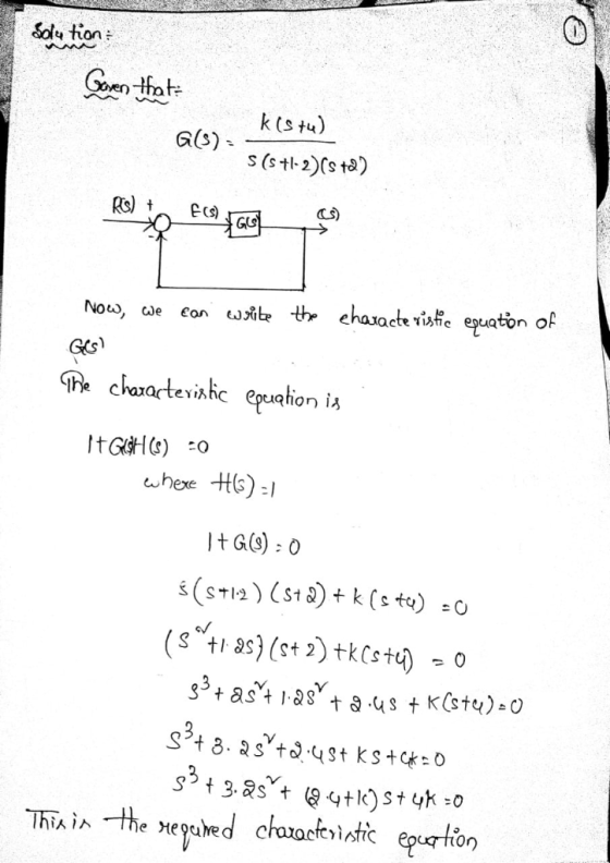
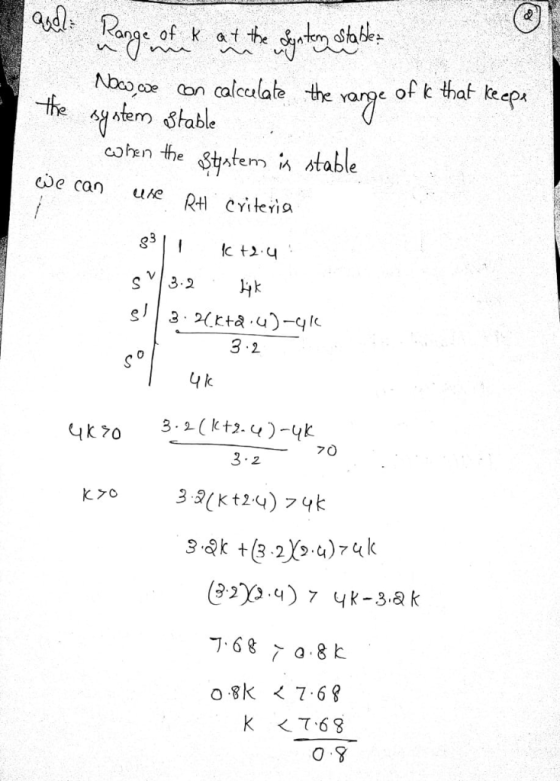
 Puge 328 polf prt 33 Question 3 [20 Marks (a) K(s+4) $(s+1)(s+2) 5 KCGTA) Given the unity-feedback system of Figure 3.1 with G(s) = do the following: T9= Construct the Routh-Hurwitz table [2 Marks] Find the range of K that keeps the system stable i. (2 Marks] Find the Value of K that makes the system oscillate [2 Marks iv. find the frequency of oscillation when K is set to the value akes the (4 Marks system oscillate R(S) E(s)...
Consider the unity feedback system is given below R(S) C(s) G() with transfer function: G(s) =...
 Consider the unity feedback system is given below R(S) C(s) G() with transfer function: G(s) = K s(s + 1)(s + 2)(8 + 6) a) Find the value of the gain K, that will make the system stable. b) Find the value of the gain K, that will make the system marginally stable. c) Find the actual location of the closed-loop poles when the system is marginally stable.
Problem 2: For a unity feedback system where the plant is defined as G(s) K s(s+3)(s...
 Problem 2: For a unity feedback system where the plant is defined as G(s) K s(s+3)(s +5) a. Sketch the Nyquist Counter path and Nyquist diagram. Clearly show the real and imag- inary axis intercept points and the low and high frequency asymptotes. (10 pts) b. Using the Nyquist criterion, obtain the range of K in which the system can be stable, unstable, and also find the value of gain K for marginal stability. (7 pts) c. Calculate the frequency...
1. Given the unity feedback system, where K(s+1(s 2) 1)(s-4) G(s) do the following: (a) Find the ...
 1. Given the unity feedback system, where K(s+1(s 2) 1)(s-4) G(s) do the following: (a) Find the root locus form. (b) Sketch the root locus. (c) Find the value of K such that the system is stable. (d) Find one value of K such that the closed-loop has a settling time less than or equal to 4 second and the percent of overshoot is less than or equal to 10 with the aid of MATLAB
1. Given the unity feedback...
1. Given the unity feedback system, where K(s+1(s 2) 1)(s-4) G(s) do the following: (a) Find the root locus form. (b) Sketch the root locus. (c) Find the value of K such that the system is stable. (d) Find one value of K such that the closed-loop has a settling time less than or equal to 4 second and the percent of overshoot is less than or equal to 10 with the aid of MATLAB
1. Given the unity feedback...
Consider the unity feedback system is given below R(S) C(s) G(s) with transfer function: G() =...
 Consider the unity feedback system is given below R(S) C(s) G(s) with transfer function: G() = K(+2) s(s+ 1/s + 3)(+5) a) Sketch the root locus. Clearly indicate any asymptotes. b) Find the value of the gain K, that will make the system marginally stable. c) Find the value of the gain K, for which the closed-loop transfer function will have a pole on the real axis at (-0.5).
3. Consider a unity feedback system with G(s)=- s(s+1)(s+2) a) Sketch the bode plot and find...
 3. Consider a unity feedback system with G(s)=- s(s+1)(s+2) a) Sketch the bode plot and find the phase margin, gain crossover frequency, gain margin, and phase crossover frequency. b) Suppose G(s) is replaced with — - Kets s(s+1)(s+2) i. For the phase margin you have computed in (a), find the minimum value for t that makes the system marginally stable. Suppose t is 1 second. What is the range of K for stability? (You can use MATLAB for this part.)...
Automatic Control In unity feedback system with Gs) (s-IXs-2) With out controller, is this system stable, and why? For Gc K (proportional control) sketch the root locus. Find the range of K to mak...
 Automatic Control
In unity feedback system with Gs) (s-IXs-2) With out controller, is this system stable, and why? For Gc K (proportional control) sketch the root locus. Find the range of K to make the system stable. Determine the range of K, so that the system has no overshoot Determine the range of K for steady state error to unit step input less than 20% a) b) c) d) e)
In unity feedback system with Gs) (s-IXs-2) With out controller,...
Automatic Control
In unity feedback system with Gs) (s-IXs-2) With out controller, is this system stable, and why? For Gc K (proportional control) sketch the root locus. Find the range of K to make the system stable. Determine the range of K, so that the system has no overshoot Determine the range of K for steady state error to unit step input less than 20% a) b) c) d) e)
In unity feedback system with Gs) (s-IXs-2) With out controller,...
For the unity feedback system, where G(s) =-s-2)(s-1) make an accurate plot of the root locus...
 For the unity feedback system, where G(s) =-s-2)(s-1) make an accurate plot of the root locus and find the following: (a) The breakaway and break-in points (b) The range of K to keep the system stable (c) The value of K that yields a stable system with critically damped second-order poles (d) The value of K that yields a stable system with a pair of second-order poles that have a damping ratio of 0.707
3. Given the unity feedback system, where G(s) = s(s +2) (s+3)(s +4) do the following:...
 3. Given the unity feedback system, where G(s) = s(s +2) (s+3)(s +4) do the following: (a) Sketch the root locus (b) Find the asymptotes c) Find the value of gain that will make the system marginally stable (d) Find the value of gain for which the closed-loop transfer function will have a pole on the real axis at-0.5
 Given the unity feedback system of Figure 1, find the following The range of K that keeps the system stable The value of K that makes the system oscillate The frequency of oscillation when K is set to the value that makes the system oscillate with: K(s-1)(s-2) (s+2)(s2+2s + 2) G(s) C(s) R(s) E(s) + G(s) Figure: 1
Given the unity feedback system of Figure 1, find the following The range of K that keeps the system stable The value...
Given the unity feedback system of Figure 1, find the following The range of K that keeps the system stable The value of K that makes the system oscillate The frequency of oscillation when K is set to the value that makes the system oscillate with: K(s-1)(s-2) (s+2)(s2+2s + 2) G(s) C(s) R(s) E(s) + G(s) Figure: 1
Given the unity feedback system of Figure 1, find the following The range of K that keeps the system stable The value...
 Puge 328 polf prt 33 Question 3 [20 Marks (a) K(s+4) $(s+1)(s+2) 5 KCGTA) Given the unity-feedback system of Figure 3.1 with G(s) = do the following: T9= Construct the Routh-Hurwitz table [2 Marks] Find the range of K that keeps the system stable i. (2 Marks] Find the Value of K that makes the system oscillate [2 Marks iv. find the frequency of oscillation when K is set to the value akes the (4 Marks system oscillate R(S) E(s)...
 Consider the unity feedback system is given below R(S) C(s) G() with transfer function: G(s) = K s(s + 1)(s + 2)(8 + 6) a) Find the value of the gain K, that will make the system stable. b) Find the value of the gain K, that will make the system marginally stable. c) Find the actual location of the closed-loop poles when the system is marginally stable.
 Problem 2: For a unity feedback system where the plant is defined as G(s) K s(s+3)(s +5) a. Sketch the Nyquist Counter path and Nyquist diagram. Clearly show the real and imag- inary axis intercept points and the low and high frequency asymptotes. (10 pts) b. Using the Nyquist criterion, obtain the range of K in which the system can be stable, unstable, and also find the value of gain K for marginal stability. (7 pts) c. Calculate the frequency...
 1. Given the unity feedback system, where K(s+1(s 2) 1)(s-4) G(s) do the following: (a) Find the root locus form. (b) Sketch the root locus. (c) Find the value of K such that the system is stable. (d) Find one value of K such that the closed-loop has a settling time less than or equal to 4 second and the percent of overshoot is less than or equal to 10 with the aid of MATLAB
1. Given the unity feedback...
1. Given the unity feedback system, where K(s+1(s 2) 1)(s-4) G(s) do the following: (a) Find the root locus form. (b) Sketch the root locus. (c) Find the value of K such that the system is stable. (d) Find one value of K such that the closed-loop has a settling time less than or equal to 4 second and the percent of overshoot is less than or equal to 10 with the aid of MATLAB
1. Given the unity feedback...
 Consider the unity feedback system is given below R(S) C(s) G(s) with transfer function: G() = K(+2) s(s+ 1/s + 3)(+5) a) Sketch the root locus. Clearly indicate any asymptotes. b) Find the value of the gain K, that will make the system marginally stable. c) Find the value of the gain K, for which the closed-loop transfer function will have a pole on the real axis at (-0.5).
 3. Consider a unity feedback system with G(s)=- s(s+1)(s+2) a) Sketch the bode plot and find the phase margin, gain crossover frequency, gain margin, and phase crossover frequency. b) Suppose G(s) is replaced with — - Kets s(s+1)(s+2) i. For the phase margin you have computed in (a), find the minimum value for t that makes the system marginally stable. Suppose t is 1 second. What is the range of K for stability? (You can use MATLAB for this part.)...
 Automatic Control
In unity feedback system with Gs) (s-IXs-2) With out controller, is this system stable, and why? For Gc K (proportional control) sketch the root locus. Find the range of K to make the system stable. Determine the range of K, so that the system has no overshoot Determine the range of K for steady state error to unit step input less than 20% a) b) c) d) e)
In unity feedback system with Gs) (s-IXs-2) With out controller,...
Automatic Control
In unity feedback system with Gs) (s-IXs-2) With out controller, is this system stable, and why? For Gc K (proportional control) sketch the root locus. Find the range of K to make the system stable. Determine the range of K, so that the system has no overshoot Determine the range of K for steady state error to unit step input less than 20% a) b) c) d) e)
In unity feedback system with Gs) (s-IXs-2) With out controller,...
 For the unity feedback system, where G(s) =-s-2)(s-1) make an accurate plot of the root locus and find the following: (a) The breakaway and break-in points (b) The range of K to keep the system stable (c) The value of K that yields a stable system with critically damped second-order poles (d) The value of K that yields a stable system with a pair of second-order poles that have a damping ratio of 0.707
 3. Given the unity feedback system, where G(s) = s(s +2) (s+3)(s +4) do the following: (a) Sketch the root locus (b) Find the asymptotes c) Find the value of gain that will make the system marginally stable (d) Find the value of gain for which the closed-loop transfer function will have a pole on the real axis at-0.5
Most questions answered within 3 hours.
-
Let X be a continuous random variable whose PDF is Let X be a
continuous random...
asked 4 minutes ago -
Martinez Company’s relevant range of production is 7,500 units
to 12,500 units. When it produces and...
asked 2 minutes ago -
A football with a mass of 1.2 kg is kicked from ground level to
a height...
asked 8 minutes ago -
Remember: Changes in supply determinants shift supply, and
changes in demand determinants shift demand. We say...
asked 6 minutes ago -
Why is the answer b), for this question? I came up with C) for
my incorrect...
asked 12 minutes ago -
Suppose that you know that in the population of full-time
employees in the United States, the...
asked 34 minutes ago -
This experiment was designed originally to sample various meat and carcass quality
aspects of Ontario pigs...
asked 35 minutes ago -
Dopamine Hydrochloride: draw the structure And Show the
functional groups in different colors and label the...
asked 27 minutes ago -
A rope supports a 10 kg dumbbell hanging from it. What is the
tension in the...
asked 26 minutes ago -
) Raw materials are studied for contamination. Suppose that
the number of particles of contamination per...
asked 49 minutes ago -
After running a regression analysis we calculated an F test and
the significance level was 0.15....
asked 45 minutes ago -
----Can someone please help me solve this one using JAVA
----I thank you in advance
Create...
asked 49 minutes ago